4. Quick Start

This section will cover in turn:

How to install Docker on different system environments
How to start a Docker container
How to convert onnx models to joint models using the Pulsar Docker toolchain
How to use joint models to run emulations on x86 platforms
How to measure the degree of difference between the inference results of joint and the inference results of onnx (internally called pairwise splitting)

The onboard speed of the model mentioned in this section is based on the toolchain axera_neuwizard_v0.6.1.14.tar.gz compiled and generated, and is not used as a basis for actual performance evaluation.

Note

The so-called pairwise splitting, i.e., comparing the error between the inference results of different versions (file types) of the same model before and after the toolchain is compiled.

4.1. Development Environment Preparation

This section describes the development environment preparation before using the Pulsar toolchain.

Pulsar uses Docker containers for toolchain integration. Users can load Pulsar image files through Docker and then perform model conversion, compilation, simulation, etc. Therefore, the development environment preparation stage only requires the correct installation of the Docker environment. Supported systems MacOS, Linux, Windows.

4.1.1. Installing the Docker development environment

After Docker is successfully installed, type sudo docker -v

$ sudo docker -v
Docker version 20.10.7, build f0df350

If the above is displayed, it means Docker has been installed successfully. The following section describes the installation and startup of the Pulsar toolchain Image.

4.1.2. Installing the Pulsar toolchain

The installation of the Pulsar toolchain is illustrated with the system version Ubuntu 18.04 and the toolchain axera_neuwizard_v0.6.1.44.tar.gz. Toolchain access.

Obtain from the AXera-Pi developer community.
Released by AXera technical support after signing an NDA with them through the corporate channel.

4.1.2.1. Loading Docker Image

Unzip axera_neuwizard_v0.6.1.14.tar.gz and enter the axera_neuwizard_v0.6.1.14 directory, run the install.sh script, and load the toolchain image file. The code example is as follows:

$ tar -xvf axera_neuwizard_v0.6.1.14.tar.gz
$ cd axera_neuwizard_v0.6.1.14
$ ls .
axera_neuwizard_0.6.1.14.tgz  install.sh  VERSION
$ sudo ./install.sh

where install.sh is an executable script that loads the .tgz image file. Importing the image file correctly will print the following log:

$ sudo ./install.sh
0e4056611adc: Loading layer [==================================================]  243.7MB/243.7MB
e4ff4d6a40b8: Loading layer [==================================================]   2.56kB/2.56kB
a162c244071d: Loading layer [==================================================]  3.072kB/3.072kB
564c200efe9b: Loading layer [==================================================]  4.608kB/4.608kB
b945acdca3b6: Loading layer [==================================================]  6.144kB/6.144kB
ee6ebe7bedc1: Loading layer [==================================================]   5.12kB/5.12kB
45f02a0e56e2: Loading layer [==================================================]  2.048kB/2.048kB
9758fe1f19bd: Loading layer [==================================================]   2.56kB/2.56kB
Loaded image: axera/neuwizard:0.6.1.14

When finished, run sudo docker image ls

$ sudo docker image ls
# Print the following data
REPOSITORY TAG IMAGE ID CREATED SIZE
axera/neuwizard 0.6.1.14 2124c702c879 3 weeks ago 3.24GB

You can see that the toolchain image has been loaded successfully, and you can start the container based on it.

4.1.2.2. Launch Toolchain Mirror

Attention

The Pulsar toolchain is built on Docker containers and requires a high level of memory on the physical machine, usually at least 32G or more is recommended, If the memory is not enough during the model conversion, neuwizard killed by SIGKILL error may occur.

Execute the following command to start the Docker container, and enter the bash environment after a successful run

$ sudo docker run --it --net host --rm --shm-size 32g -v $PWD:/data axera/neuwizard:0.6.1.14

The -shm-size parameter is recommended to be set to 32g and above, and the -v parameter controls the mapping of the external folder to the internal folder of the container, for example $PWD:/data means the current folder is mapped to the /data folder in the container.

4.2. Model compilation and simulation, as well as the description of the pair of scores

This section describes the basic operation of ONNX model conversion, using the pulsar tool to compile ONNX models into joint models. Please refer to the Development Environment Preparation section to complete the development environment. The example model in this section is the open source model ResNet18.

4.2.1. Data preparation

Hint

The model ResNet18 and related dependencies for this section are provided in the quick_start_example folder quick_start_example.zip Downloaded from Then unzip the downloaded file and copy it to docker under the /data path.

After successfully starting the toolchain image, copy the five folders from quick_start_example.zip to the /data folder, and then execute

root@xxx:/data# ls
config dataset gt images model

The model folder holds the ONNX model files to be compiled, and the dataset holds the Calibration dataset for the PTQ (Post-Training Quantization) (the dataset is packaged in .tar format), The config folder is used to store the configuration files needed to compile the model, gt is used to store the results of the simulation runs, and images is used to store the test images.

After the data preparation, the directory tree structure is as follows:

root@xxx:/data# tree
.
├── config
│   └── config_resnet18.prototxt
├── dataset
│   └── imagenet-1k-images.tar
├── gt
├── images
│   ├── cat.jpg
│   ├── img-319.jpg
│   ├── img-416.jpg
│   └── img-642.jpg
└── model
    └── resnet18.onnx

Hint

The tree command is not pre-installed in the toolchain docker, and can be viewed outside of docker.

4.2.2. Command description

The functional commands in the Pulsar toolchain start with pulsar, and the user-strong related commands are pulsar build , `pulsar run and pulsar version.

pulsar build is used to convert onnx models to joint format models
pulsar run is used for joint validation before and after model conversion
pulsar version can be used to see the current version of the toolchain, which is usually required for feedback issues

root@xxx:/data# pulsar --help
usage: pulsar [-h] {debug,build,version,info,run,view} ...

positional arguments:
{debug,build,version,info,run,view}
    debug               score compare debug tool
    build               from onnx to joint
    version             version info
    info                brief model
    run                 simulate models
    view                neuglass to visualize mermaids

optional arguments:
-h, --help            show this help message and exit

4.2.3. Configuration file description

config_resnet18.prototxt under the /data/config/ path Show:

# Basic configuration parameters: input and output
input_type: INPUT_TYPE_ONNX
output_type: OUTPUT_TYPE_JOINT

# Hardware platform selection
target_hardware: TARGET_HARDWARE_AX620

# CPU backend selection, default is AXE
cpu_backend_settings {
    onnx_setting {
        mode: DISABLED
    }
    axe_setting {
        mode: ENABLED
        axe_param {
            optimize_slim_model: true
        }
    }
}

# Model input data type settings
src_input_tensors {
    color_space: TENSOR_COLOR_SPACE_RGB
}

dst_input_tensors {
    color_space: TENSOR_COLOR_SPACE_RGB
    # color_space: TENSOR_COLOR_SPACE_NV12 # If the input data is NV12, then this configuration is used
}

# Configuration parameters for the neuwizard tool
neuwizard_conf {
    operator_conf {
        input_conf_items {
            attributes {
                input_modifications {
                    affine_preprocess {
                        slope: 1
                        slope_divisor: 255
                        bias: 0
                    }
                }
                input_modifications {
                    input_normalization {
                        mean: [0.485,0.456,0.406]  ## mean
                        std: [0.229,0.224,0.255]   ## std
                    }
                }
            }
        }
    }
    dataset_conf_calibration {
        path: "... /dataset/imagenet-1k-images.tar" # Set the path to the PTQ calibration dataset
        type: DATASET_TYPE_TAR # dataset type: tarball
        size: 256 # The actual number of images used in the quantitative calibration process
        batch_size: 1
    batch_size: 1}

    dataset_conf_error_measurement {
        path: "... /dataset/imagenet-1k-images.tar"
        type: DATASET_TYPE_TAR # Dataset type: tarball
        size: 4 # The actual number of images used in the layer-by-layer pairing process
    }

    evaluation_conf {
        path: "neuwizard.evaluator.error_measure_evaluator"
        type: EVALUATION_TYPE_ERROR_MEASURE
        source_ir_types: IR_TYPE_ONNX
        ir_types: IR_TYPE_LAVA
        score_compare_per_layer: true
    }
}

# Output layout settings, NHWC is recommended for faster speed
dst_output_tensors {
    tensor_layout:NHWC
tensor_layout:NHWC }

# configuration parameters for pulsar compiler
pulsar_conf {
    ax620_virtual_npu: AX620_VIRTUAL_NPU_MODE_111 # business scenario requires the use of ISP, then the vNPU 111 configuration must be used, 1.8Tops arithmetic power to the user's algorithm model
    batch_size: 1
    debug : false
}

4.2.4. Model Compilation

Take resnet18.onnx as an example, execute the following pulsar build command in docker to compile resnet18.joint:

# Model conversion commands, which can be copied and run directly
pulsar build --input model/resnet18.onnx --output model/resnet18.joint --config config/config_resnet18.prototxt --output_config config/output_config.prototxt

log reference information

root@662f34d56557:/data# pulsar build --input model/resnet18.onnx --output model/resnet18.joint --config config/config_resnet18.prototxt --output_config config/output_config.prototxt

[W Context.cpp:69] Warning: torch.set_deterministic is in beta, and its design and  functionality may change in the future. (function operator())
[09 06:46:16 frozen super_pulsar.proto.configuration_super_pulsar_manip:229] set task task_0's pulsar_conf.output_dir as /data
[09 06:46:17 frozen super_pulsar.func_wrappers.wrapper_pulsar_build:28] planning task task_0
[09 06:46:17 frozen super_pulsar.func_wrappers.wrapper_pulsar_build:334] #################################### Running task task_0 ####################################
[09 06:46:17 frozen super_pulsar.toolchain_wrappers.wrapper_neuwizard:31] python3 /root/python_modules/super_pulsar/super_pulsar/toolchain_wrappers/wrapper_neuwizard.py --config /tmp/tmpa18v1l0m.prototxt
[09 06:53:25 frozen super_pulsar.toolchain_wrappers.wrapper_neuwizard:37] DBG [neuwizard] ONNX Model Version 7 for "/data/model/resnet18.onnx"
... ...
[09 07:10:33 frozen super_pulsar.toolchain_wrappers.wrapper_toolchain:482] File saved: /data/model/resnet18.joint
[09 07:10:33 frozen super_pulsar.toolchain_wrappers.wrapper_toolchain:489] DBG cleared /root/tmpxd2caw3b

Attention

resnet18.onnx model in hardware configuration of:

Intel(R) Xeon(R) Gold 6130 CPU @ 2.10GHz

Memory 32G

The conversion time on a server with Intel(R) Xeon(R) Gold 6130 CPU @ 2.10GHz Memory 32G is about 3min, which may vary from machine to machine, so be patient.

4.2.5. Upper board speed measurement

The resnet18.joint model generated during the pulsar build phase can be speed tested on the community board AX-Pi <https://item.taobao.com/item.htm?_u=m226ocm5e25&id=682169792430>`_ or the official EVB using the ``run_joint command, as follows:

First connect to the AX-Pi via ssh or serial communication.
Then copy or mount the resnet18.joint model to any folder on the development board.
Finally execute the command run_joint resnet18.joint --repeat 100 --warmup 10

Resnet18 speed log example

$ run_joint resnet18.joint --repeat 100 --warmup 10
run joint version: 0.5.10

virtual npu mode is 1_1

tools version: 0.6.1.4
59588c54
Using wbt 0
Max Batch Size 1
Support Dynamic Batch? No
Is FilterMode? No

Quantization Type is 8 bit

Input[0]: data
    Shape [1, 224, 224, 3] NHWC uint8 RGB
    Memory Physical
    Size 150528
Output[0]: resnetv15_dense0_fwd
    Shape [1, 1000] NHWC float32
    Memory Physical
    Size 4000

Using batch size 1
input[0] data data not provided, using random data

Not set environment variable to report memory usage!

CMM usage: 13761984

Create handle took 569.69 ms (neu 10.77 ms, onnx 0.00 ms, axe 0.00 ms, overhead 558.93 ms)
Run task took 5415 us (99 rounds for average)
        Run NEU took an average of 5378 us (overhead 10 us)

NPU perf cnt total: 4190383
        NPU perf cnt of eu(0): 2543447
        NPU perf cnt of eu(1): 0
        NPU perf cnt of eu(2): 0
        NPU perf cnt of eu(3): 2645657
        NPU perf cnt of eu(4): 0

Hint

In the above log, the NPU inference time for resnet18 is 5.415ms (the NEU file is executed on the NPU), no CPU time is consumed, overhead is the time used for model decompression, parsing, loading and memory allocation, which is initialized only once and can be ignored in real applications.

In some cases, the transformed model will contain a CPU tail (a DAG subgraph running on the CPU that ends in .onnx or .axe), and an example of a model speed log with a CPU tail is shown below:

$ run_joint resnet50.joint --repeat 100 --warmup 10
run joint version: 0.5.13

virtual npu mode is 1_1
tools version: 0.5.34.2
7ca3b9d5
Using wbt 0
Max Batch Size 1
Support Dynamic Batch? No
Is FilterMode? No

Quantization Type is unknown

Input[0]: data
    Shape [1, 224, 224, 3] NHWC uint8 BGR
    Memory Physical
    Size 150528
Output[0]: resnetv24_dense0_fwd
    Shape [1, 1000] NCHW float32
    Memory Virtual
    Size 4000

Using batch size 1
input[0] data data not provided, using random data

Create handle took 1830.94 ms (neu 44.76 ms, onnx 0.00 ms, axe 13.89 ms, overhead 1772.28 ms)
Run task took 32744 us (99 rounds for average)
    Run NEU took an average of 32626 us (overhead 22 us)
    Run AXE took an average of 43 us (overhead 4 us)

From the above example, we can see that NPU inference time is 32.626ms, CPU time is 43us, and the total time of model inference is the sum of NPU time and CPU time, which is 32.744ms. (P.S.: The network structure of resnet50 in this example has been modified to demonstrate the functionality of the heterogeneous cut map, and is not used as a reference for resnet50 speed evaluation)

run_joint command description

$ run_joint -h
undefined short option: -h
usage: run_joint [options] ... joint-file
options:
    --mode                   NPU mode, disable for no virtual npu; 1_1 for AX_NPU_VIRTUAL_1_1 (string [=])
-d, --data                   The format is file0;file1... to specify data files for input vars.
    'file*' would be directly loaded in binary format to tensor in order (string [=])
    --bin-out-dir            Dump output tensors in binary format (string [=])
    --repeat                 Repeat times for inference (int [=1])
    --warmup                 Repeat times for warmup (int [=0])
    --stride_w               mock input data with extra width stride (int [=0])
    --override_batch_size    override batch size for dynamic batch model (int [=0])
    --wbt_index              select WBT for inference (int [=0])
-p, --manual_alloc           manually alloc buffer with ax sys api instead of joint api
-t, --enable_trunc           truncate input data size to model required size when using a larger input data, experimental function, will be removed in future release
    --cache-mode             'CACHED' means use only cached CMM memory; 'NONE-CACHED' means use only none-cached CMM memory; 'SMART_CACHED' means use cached and none-cached CMM memory in turn (string [=CACHED])
-?, --help                   print this message

4.2.6. x86 emulation run and pair splitting instructions

Attention

Note, this section is based on the toolchain axera_neuwizard_v0.6.1.14, which is available in different versions, The command parameters may be different in different versions, so use the pulsar run -h command to see the list of command input parameters. Other commands can be used to view the argument list in the same way.

Executing the pulsar run command in docker gives you the inference results of the onnx and joint models and the degree of difference between the model outputs:

# Model emulation and pair splitting instructions, can be directly copied and run
pulsar run model/resnet18.onnx model/resnet18.joint --input images/img-319.jpg --config config/output_config.prototxt --output_gt gt/

log information reference

root@662f34d56557:/data# pulsar run model/resnet18.onnx model/resnet18.joint --input images/img-319.jpg --config config/output_config.prototxt --output_gt gt/

...
...
[26 07:14:45 <frozen super_pulsar.func_wrappers.wrapper_pulsar_run>:138] =========================

[26 07:14:45 <frozen super_pulsar.func_wrappers.pulsar_run.utils>:70] dumpped 'resnetv15_dense0_fwd' to 'gt/joint/resnetv15_dense0_fwd.bin'.
[26 07:14:45 <frozen super_pulsar.func_wrappers.pulsar_run.compare>:97] ###### Comparing resnet18.onnx (with conf) and resnet18.joint ######
[26 07:14:45 <frozen super_pulsar.func_wrappers.pulsar_run.compare>:82] Score compare table:
---------------------------  ----------------  ------------------
Layer: resnetv15_dense0_fwd  2-norm RE: 4.70%  cosine-sim: 0.9989

The layer_name, L2 regularization and cosine similarity of the model output can be obtained from the output log. The cosine similarity (cosine-sim) results provide a visualization of the loss of model accuracy (essentially comparing the difference between the inference results of the onnx and joint models).

4.2.6.1. Output file description

A description of the file generated after executing the pulsar build and pulsar run commands:

root@xxx:/data# tree

.
├── config
│   ├── config_resnet18.prototxt  # Model compilation configuration file
│   └── output_config.prototxt    # pulsar run required configuration files
├── dataset
│   └── imagenet-1k-images.tar    # Calibration data set
├── gt                            # Input data that can be used to run the demo on the board
│   ├── input
│   │   ├── data.bin
│   │   ├── data.npy
│   │   └── filename.txt
│   ├── joint                     # output data from joint model simulation runs
│   │   ├── resnetv15_dense0_fwd.bin
│   │   └── resnetv15_dense0_fwd.npy
│   └── onnx                      # Output data from the onnx model simulation run
│       ├── resnetv15_dense0_fwd.bin
│       └── resnetv15_dense0_fwd.npy
├── images                        # Test images
│   ├── cat.jpg
│   ├── img-319.jpg
│   ├── img-416.jpg
│   └── img-642.jpg
├── inference_report
│   └── part_0.lava
│       ├── inference_report.log
│       ├── subgraph_0
│       │   └── inference_report.log
│       └── subgraph_1
│           └── inference_report.log
└── model
    ├── model.lava_joint
    ├── resnet18.joint            # Compile-generated Joint model
    └── resnet18.onnx             # Original ONNX model

12 directories, 20 files

Hint

The gt folder of the pulsar run output holds the simulation inference results for the onnx and joint models, which can be used to manually map (between the joint simulation results on the x86 platform and the onboard output) and parse the output of the joint models.

4.2.6.2. Parsing the inference results of the `joint` model

The gt file tree is as follows:

$ tree gt
gt
├── input  # input data for onnx and joint models
│   ├── data.bin
│   ├── data.npy
│   └── filename.txt
├── joint  # Inference results for the joint model
│   ├── resnetv15_dense0_fwd.bin
│   └── resnetv15_dense0_fwd.npy
└── onnx  # Inference results for the onnx model
    ├── resnetv15_dense0_fwd.bin
    └── resnetv15_dense0_fwd.npy

3 directories, 7 files

The input data of the model is given in the input folder, in two forms: .bin and .npy, containing the same data information.
The inference results of the model are given in the onnx and joint folders, respectively, and the output of the model can be processed to meet different needs.

The following is an example of how to process the inference results of resnet18 model, which has the following output structure:

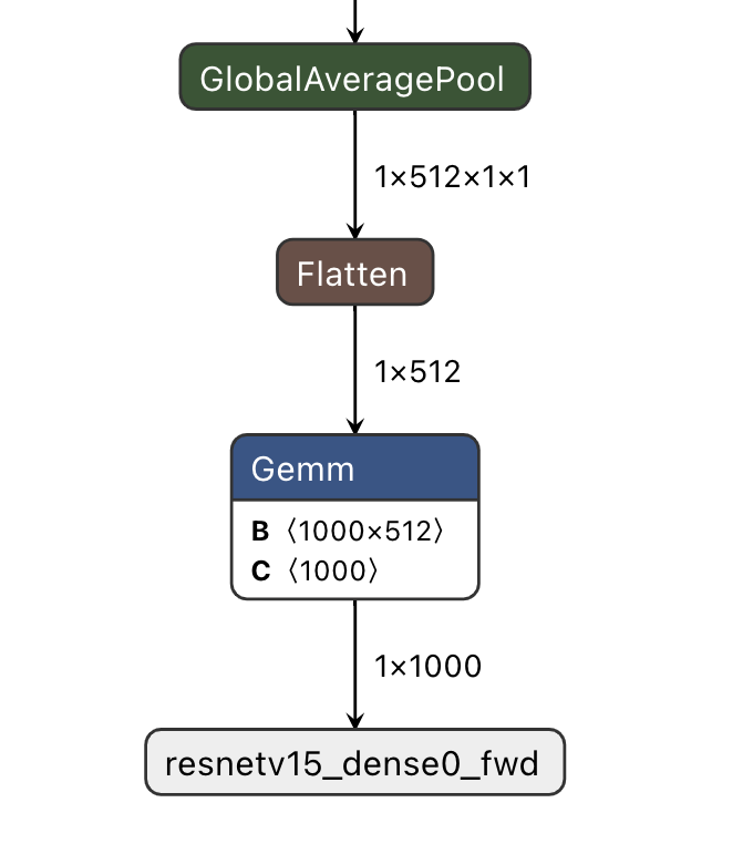
The sample code (parse_gt.py) for outputting the classification result with shape (1, 1000) is as follows:

#!/usr/bin/env python3
import math
import numpy as np
import json
import logging


# Note: The sample code is based on the resnet18 model, other models can be modified as appropriate
if __name__ == '__main__':
    import argparse
    parser = argparse.ArgumentParser()
    parser.add_argument(dest='npy', nargs="+", help='pulsar run, gt, npy file')
    parser.add_argument('--K', type=int, default=5, help='top k')
    parser.add_argument('--rtol', type=float, default=1e-2, help='relative tolerance')
    parser.add_argument('--atol', type=float, default=1e-2, help='absolute tolerance')
    args = parser.parse_args()

    assert len(args.npy) <= 2
    with open('./imagenet1000_clsidx_to_labels.json', 'r') as f:
        # imagenet1000_clsidx_to_labels: https://gist.github.com/yrevar/942d3a0ac09ec9e5eb3a
        js = f.read()
        imgnet1000_clsidx_dict = json.loads(js)

    for npy in args.npy:
        result = np.load(npy)
        indices = (-result[0]).argsort()[:args.K]
        logging.warning(f"{npy}, imagenet 1000 class index, top{args.K} result is {indices}")

        for idx in indices:
            logging.warning(f"idx: {idx}, classification result: {imgnet1000_clsidx_dict[str(idx)]}")

    if len(args.npy) == 2:  # Pair the two npy's, no output, then the pairing is successful
        npy1 = np.load(args.npy[0])
        npy2 = np.load(args.npy[1])
        assert not math.isnan(npy1.sum()) and not math.isnan(npy2.sum())
        try:
            if npy1.dtype == np.float32:
                assert np.allclose(npy1, npy2, rtol=args.rtol, atol=args.atol), "mismatch {}".format(abs(npy1 - npy2).max())
            else:
                assert np.all(npy1 == npy2), "mismatch {}".format(abs(npy1 - npy2).max())
        except AssertionError:
            logging.warning("abs(npy1 - npy2).max() = ", abs(npy1 - npy2).max())

By executing the following commands

python3 parse_gt.py  gt/onnx/resnetv15_dense0_fwd.npy gt/joint/resnetv15_dense0_fwd.npy --atol 100000 --rtol 0.000001

Example of output results:

WARNING:root:gt/onnx/resnetv15_dense0_fwd.npy, imagenet 1000 class index, top5 result is [924 948 964 935 910]
WARNING:root:idx: 924, classification result: guacamole
WARNING:root:idx: 948, classification result: Granny Smith
WARNING:root:idx: 964, classification result: potpie
WARNING:root:idx: 935, classification result: mashed potato
WARNING:root:idx: 910, classification result: wooden spoon

WARNING:root:gt/joint/resnetv15_dense0_fwd.npy, imagenet 1000 class index, top5 result is [924 948 935 964 910]
WARNING:root:idx: 924, classification result: guacamole
WARNING:root:idx: 948, classification result: Granny Smith
WARNING:root:idx: 935, classification result: mashed potato
WARNING:root:idx: 964, classification result: potpie
WARNING:root:idx: 910, classification result: wooden spoon

Hint

parse_gt.py supports parsing two npy. If no parsing log is output after execution, the parsing is successful.

4.2.6.3. Instructions for `gt` file splitting

Hint

Manual bisection is generally not necessary, and the loss of model accuracy can be easily observed by observing cosine-sim with pulsar run.

Manual alignment requires building the alignment script manually, as described below:

# Create the script file used for the score

$ vim compare_fp32.py

compare_fp32.py reads as follows:

#!/usr/bin/env python3
import math
import numpy as np

if __name__ == '__main__':
    import argparse
    parser = argparse.ArgumentParser()
    parser.add_argument(dest='bin1', help='bin file as fp32')
    parser.add_argument(dest='bin2', help='bin file as fp32')
    parser.add_argument('--rtol', type=float, default=1e-2,
                        help='relative tolerance')
    parser.add_argument('--atol', type=float, default=1e-2,
                        help='absolute tolerance')
    parser.add_argument('--report', action='store_true', help='report for CI')
    args = parser.parse_args()

    try:
        a = np.fromfile(args.bin1, dtype=np.float32)
        b = np.fromfile(args.bin2, dtype=np.float32)
        assert not math.isnan(a.sum()) and not math.isnan(b.sum())
    except:
        a = np.fromfile(args.bin1, dtype=np.uint8)
        b = np.fromfile(args.bin2, dtype=np.uint8)
    try:
        if a.dtype == np.float32:
            assert np.allclose(a, b, rtol=args.rtol, atol=args.atol), "mismatch {}".format(abs(a - b).max())
        else:
            assert np.all(a == b), "mismatch {}".format(abs(a - b).max())
        if args.report:
            print(0)
    except AssertionError:
        if not args.report:
            raise
        else:
            print(abs(a - b).max())

After the script is created successfully, execute the following command to get the joint model results in the actual board:

run_joint resnet18.joint --data gt/input/data.bin --bin-out-dir out/ --repeat 100

The joint upboarding results are saved in the out folder.

$ python3 compare_fp32.py --atol 100000 --rtol 0.000001 gt/joint/resnetv24_dense0_fwd.bin out/resnetv24_dense0_fwd.bin

After executing the command, no result is returned, which means the pairing is successful.

4.3. Development board running

This section describes how to run the resnet18.joint model on the AX-Pi development board, obtained via the Model Compile Simulation section. The example shows how a classification network can classify an input image, but more specifically, for example, the source code of the open source project ax-samples is compiled to generate an executable For other examples (object detection, image segmentation, human keypoints, etc.), please refer to the Detailed description of model deployment section.

4.3.1. Development Board Acquisition

Acquired through AX-Pi designated Taobao Mall (Purchase link);
Get EVB after signing the NDA with AXera through the corporate channel.

4.3.2. Data preparation for onboard operation

Hint

The upper board runtime example has been packaged in the demo_onboard folder demo_onboard.zip download link Extract the downloaded file, where ax_classification is the pre-cross-compiled classification model executable that can be run on the AX-Pi development board. resnet18.joint is the compiled classification model, and cat.jpg is the test image.

Copy ax_classification, resnet18.joint, and cat.png to the board, and if ax_classification lacks executable permissions, you can add them with the following command

/root/sample # chmod a+x ax_classification  # Add execution rights
/root/sample # ls -l
total 15344
-rwxrwxr-x    1 1000     1000       3806352 Jul 26 15:22 ax_classification
-rw-rw-r--    1 1000     1000        140391 Jul 26 15:22 cat.jpg
-rw-rw-r--    1 1000     1000      11755885 Jul 26 15:22 resnet18.joint

4.3.3. Run `Resnet18` classification model on the board

ax_classification Input parameter description:

/root/sample # ./ax_classification --help
usage: ./ax_classification --model=string --image=string [options] ...
options:
-m, --model     joint file(a.k.a. joint model) (string)
-i, --image     image file (string)
-g, --size      input_h, input_w (string [=224,224])
-r, --repeat    repeat count (int [=1])
-?, --help      print this message

The classification model is implemented on the board by executing the ax_classification program, and the results are as follows:

/root/sample # ./ax_classification -m resnet18.joint -i cat.png -r 100
--------------------------------------
model file : resnet18.joint
image file : cat.jpg
img_h, img_w : 224 224
Run-Joint Runtime version: 0.5.10
--------------------------------------
[INFO]: Virtual npu mode is 1_1

Tools version: 0.6.1.4
59588c54
11.4611, 285
10.0656, 278
9.8469, 287
9.0733, 282
9.0031, 279
--------------------------------------
Create handle took 570.64 ms (neu 10.89 ms, axe 0.00 ms, overhead 559.75 ms)
--------------------------------------
Repeat 100 times, avg time 5.42 ms, max_time 5.81 ms, min_time 5.40 ms

4. Quick Start

4.1. Development Environment Preparation

4.1.1. Installing the Docker development environment

4.1.2. Installing the Pulsar toolchain

4.1.2.1. Loading Docker Image

4.1.2.2. Launch Toolchain Mirror

4.2. Model compilation and simulation, as well as the description of the pair of scores

4.2.1. Data preparation

4.2.2. Command description

4.2.3. Configuration file description

4.2.4. Model Compilation

4.2.5. Upper board speed measurement

4.2.6. x86 emulation run and pair splitting instructions

4.2.6.1. Output file description

4.2.6.2. Parsing the inference results of the joint model

4.2.6.3. Instructions for gt file splitting

4.3. Development board running

4.3.1. Development Board Acquisition

4.3.2. Data preparation for onboard operation

4.3.3. Run Resnet18 classification model on the board

4.2.6.2. Parsing the inference results of the `joint` model

4.2.6.3. Instructions for `gt` file splitting

4.3.3. Run `Resnet18` classification model on the board