5. Model Conversion Advanced Guide

5.1. Pulsar Build model compilation

This section describes the complete use of the pulsar build command.

5.1.1. Overview

pulsar build is used for model optimization, quantization, compilation, and other operations. A diagram of its operation is shown below:

graph LR; Input model [input model onnx] --> pb(pulsar build<br/>+command line arguments) Configuration file [config.prototxt] --> pb pb --> output model [output model joint] pb --> output configuration file [configuration file output_config.prototxt]

pulsar build takes the input model (model.onnx) and the configuration file (config.prototxt) and compiles them to get the output model (joint) and the output configuration file (output_config.prototxt).

The command line arguments of pulsar build will override some parts of the configuration file and cause pulsar build to output the overwritten configuration file. See Configuration file details for a detailed description of the configuration file.

pulsar build -h shows detailed command line arguments:

root@xxx:/data# pulsar build -h
usage: pulsar build [-h] [--config CONFIG] [--output_config OUTPUT_CONFIG]
                    [--input INPUT [INPUT ...]] [--output OUTPUT [OUTPUT ...]]
                    [--calibration_batch_size CALIBRATION_BATCH_SIZE]
                    [--compile_batch_size COMPILE_BATCH_SIZE [COMPILE_BATCH_SIZE ...]]
                    [--batch_size_option {BSO_AUTO,BSO_STATIC,BSO_DYNAMIC}]
                    [--output_dir OUTPUT_DIR]
                    [--virtual_npu {0,311,312,221,222,111,112}]
                    [--input_tensor_color {auto,rgb,bgr,gray,nv12,nv21}]
                    [--output_tensor_color {auto,rgb,bgr,gray,nv12,nv21}]
                    [--output_tensor_layout {native,nchw,nhwc}]
                    [--color_std {studio,full}]
                    [--target_hardware {AX630,AX620,AX170}]
                    [--enable_progress_bar]

optional arguments:
  -h, --help            show this help msesage and exit
  --config CONFIG       .prototxt
  --output_config OUTPUT_CONFIG
  --input INPUT [INPUT ...]
  --output OUTPUT [OUTPUT ...]
  --calibration_batch_size CALIBRATION_BATCH_SIZE
  --compile_batch_size COMPILE_BATCH_SIZE [COMPILE_BATCH_SIZE ...]
  --batch_size_option {BSO_AUTO,BSO_STATIC,BSO_DYNAMIC}
  --output_dir OUTPUT_DIR
  --virtual_npu {0,311,312,221,222,111,112}
  --input_tensor_color {auto,rgb,bgr,gray,nv12,nv21}
  --output_tensor_color {auto,rgb,bgr,gray,nv12,nv21}
  --output_tensor_layout {native,nchw,nhwc}
  --color_std {studio,full}
                        only support nv12/nv21 now
  --target_hardware {AX630,AX620,AX170}
                        target hardware to compile
  --enable_progress_bar

Hint

Complex functions can be implemented using configuration files, and command-line arguments only play a supporting role. In addition, the command line parameters override some of the corresponding configuration in the configuration file.

5.1.2. Detailed explanation of parameters

pulsar build Parameter explanation

--input

The input model path for this compilation, corresponding to the input_path field in config.prototxt

--output

Specify the file name of the output model, e.g. compiled.joint, corresponding to output_path field in config.prototxt

--config

Specifies the basic configuration file used to guide the compilation process. If command-line arguments are specified for the pulsar build command, the values specified in the command-line arguments will be used in preference to those specified in the conversion model

--output_config

Outputs the complete configuration information used in this build to a file

--target_hardware

Specify the hardware platform for compiling the output model, currently AX630 and AX620 are available

--virtual_npu

Specify the virtual NPU to be used for inference, please differentiate according to the -target_hardware parameter. See the virtual NPU section in chip_introduction for details

--output_dir

Specifies the working directory for the compilation process. The default is the current directory

--calibration_batch_size

The batch_size of the data used for internal parameter calibration in the transcoding process. The default value is 32.

--batch_size_option

Sets the batch type supported by the joint format model:

• BSO_AUTO: default option, static by default batch

• BSO_STATIC: static batch, fixed batch_size during inference, optimal performance

• BSO_DYNAMIC: dynamic batch, supports arbitrary batch_size up to the maximum value when reasoning, most flexible

--compile_batch_size

Sets the batch size supported by the joint format model. The default is 1.

• When -batch_size_option BSO_STATIC is specified, batch_size indicates the unique batch size that the joint format model can use for reasoning.

• When -batch_size_option BSO_DYNAMIC is specified, batch_size indicates the maximum batch size that can be used for joint format model inference.

--input_tensor_color

Specify the color space of input data for input model, optional:

• Default option: auto, automatic recognition based on the number of input channels to the model

  • 3-channel is bgr

  • 1-channel is gray

• Other options: rgb, bgr, gray, nv12, nv21

--output_tensor_color

Specify the color space of the input data for the output model, optional:

• Default option: auto, automatic recognition based on the number of input channels to the model

  • 3-channel is bgr

  • 1-channel is gray

• Other options: rgb, bgr, gray, nv12, nv21

--color_std

Specify the conversion standard to be used when converting between RGB and YUV, options: legacy, studio and full, default is legacy

--enable_progress_bar

Show progress bar at compile time. Not shown by default

--output_tensor_layout

Specify the layout of the output model of the tensor, optional:

• native: default option, legacy option, not recommended. It is recommended to explicitly specify the output layout

• nchw

• nhwc

Attention

This parameter is only supported by axera_neuwizard_v0.6.0.1 and later toolchains. Starting from axera_neuwizard_v0.6.0.1, the default layout of the output tensor of some AX620A models may be different from the default layout of the axera_neuwizard_v0.6.0.1. may differ from the model compiled from the toolchain of previous versions of axera_neuwizard_v0.6.0.1. The default layout of the AX630A model is not affected by the toolchain version

Code examples

pulsar build --input model.onnx --output compiled.joint --config my_config.prototxt --target_hardware AX620 --virtual_npu 111 --output_config my_output_config.prototxt

Tip

When generating joint models that support dynamic batch, multiple common batch_size can be specified after -compile_batch_size to improve performance when reasoning with batch size up to these values.

Attention

Specifying multiple batch sizes will increase the size of the joint model file.

5.2. Pulsar Run model simulation and alignment

This section describes the complete use of the pulsar run command.

5.2.1. Overview

pulsar run is used to perform x86 simulation and precision pair splitting of joint models on the x86 platform.

graph LR; Target Model[Target Model<br/>joint] --> pulsar_run(pulsar run<br/>+command line parameter) Reference Model [Reference Model<br/>onnx] --> pulsar_run Image files [Image files<br/>jpg / png] --> pulsar_run pulsar_run --> pair splitting result pulsar_run --> gt[Simulation of target model inference results<br/>+<br/>input data on board]

pulsar run -h shows detailed command line arguments:

root@xxx:/data# pulsar run -h
usage: pulsar run [-h] [--use_onnx_ir] [--input INPUT [INPUT ...]]
                  [--layer LAYER [LAYER ...]] [--output_gt OUTPUT_GT]
                  [--config CONFIG]
                  model [model ...]

positional arguments:
  model

optional arguments:
  -h, --help                   show this help msesage and exit
  --use_onnx_ir                use NeuWizard IR for refernece onnx
  --input INPUT [INPUT ...]    input paths or .json
  --layer LAYER [LAYER ...]    input layer namse
  --output_gt OUTPUT_GT        save gt data in dir
  --config CONFIG

pulsar run Parameter explanation

Required parameters

model.joint model.onnx

--input

Multiple input data can be specified and used as input data for the simulation inference. Support jpg, png, bin, etc., and make sure the number of them is the same as the number of model input layers

--layer

Not required

When the model has multiple inputs, it is used to specify which layer the input data should be on. The order is in contrast to -input.

For example, -input file1.bin file2.bin --layer layerA layerB means input file1.bin to layerA and input file2.bin to layerB, making sure that the length of -layer is the same as the length of -input.

--use_onnx_ir

This option tells pulsar run to internally infer the onnx model with NeuWizard IR when using the onnx format model as a counterpoint reference model. By default, NeuWizard IR is not used.

This option is only meaningful if `` –onnx`` is specified, it can be ignored

--output_gt

Specifies the directory where the simulation inference results of the target model and the upper board input data are stored. No output by default

--config

Specifies a configuration file to guide pulsar run in the internal conversion of the reference model. The configuration file is generally output using the -pulsar build --output_config option

pulsar run code example

pulsar run model.onnx compiled.joint --input test.jpg --config my_output_config.prototxt --output_gt gt

5.3. Pulsar Info View model information

Attention

Note: The pulsar info feature will only work with docker toolchains with version numbers greater than 0.6.1.2.

For .joint models transferred from an old toolchain, the correct information cannot be seen with pulsar info and needs to be reconverted with a newer toolchain. The reason is that the Performance.txt file in the old joint does not contain the onnx layer name information and needs to be reconverted.

pulsar info is used to view information about onnx and joint models, and supports saving model information to html, grid, jira formats.

Usage commands

pulsar info model.onnx/model.joint

Parameter list

$ pulsar info -h

usage: pulsar info [-h] [--output OUTPUT] [--output_json OUTPUT_JSON]
                  [--layer_mapping] [--performance] [--part_info]
                  [--tablefmt TABLEFMT]
                  model

positional arguments:
  model

optional arguments:
  -h, --help            show this help msesage and exit
  --output OUTPUT       path to output dir
  --output_json OUTPUT_JSON
  --layer_mapping
  --performance
  --part_info
  --tablefmt TABLEFMT   possible formats (html, grid, jira, etc.)

Parameter description

pulsar info Parameter explanation

--output

Specify the directory where the model information is saved, not saved by default

--output_json

Save the full model information as Json, not saved by default

--layer_mapping

Show layer_mapping information of Joint model, not shown by default

Can be used to see the correspondence between onnx layer and the converted lava layer

--performance

Show performance information of Joint model, not shown by default

--parts

Displays all information about each part of the Joint model, not shown by default

--tablefmt

Specify the format for displaying and saving model information, optional:

• simple: DEFAULT

• grid

• html

• jira

• … Any of the tablefmt formats supported by the tabulate library

Example: View basic model information

pulsar info resnet18.joint

# output log
[24 18:40:10 wrapper_pulsar_info.py:32] Information of resnet18.joint:
IO Meta Info:
NAME                  I/O?    SHAPE             DTYPE    LAYOUT
--------------------  ------  ----------------  -------  --------
data                  INPUT   [1, 224, 224, 3]  uint8    NHWC
resnetv15_dense0_fwd  OUTPUT  [1, 1000]         float32  NCHW

Approx System Memory: 13.84 MB
Approx Standard Memory: 0 B
Approx Memory: 13.84 MB

Virtual NPU: AX620_VNPU_111
Static Batch: 1
Toolchain Version: dfdce086b

Example: See the correspondence between the onnx layer and the layer of the compiled model

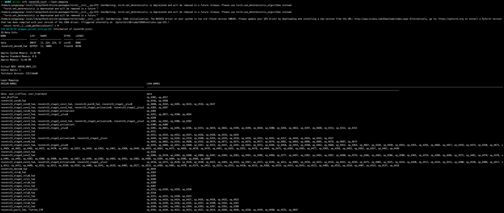
where ORIGIN_NAmse is the layer name of the original onnx, and LAVA_NAmse is the layer name of the compiled model.

Note

Specify the parameters in pulsar info:

• --layer_mapping parameter to see the correspondence between onnx_layer_name and the layer_name of the transformed model

• The --performance parameter allows you to see the performance information for each layer.

5.4. Pulsar Version View Toolchain Version

pulsar version is used to get the tool version information.

Hint

If you need to provide us with toolchain error information, please submit the version of the toolchain you are using along with the information.

Code examples

pulsar version

Example result

0.5.34.2
7ca3b9d5

5.5. Tools

The Pulsar toolchain also provides other common network model processing tools, which help users to format the network model and other functions.

5.5.1. Caffe2ONNX

The dump_onnx.sh tool is pre-installed in the Docker image of Pulsar, providing the ability to convert Caffe models to ONNX models, thus indirectly extending pulsar build support for Caffe models. This is done as follows:

dump_onnx.sh -h to display detailed command line arguments:

root@xxx:/data$ dump_onnx.sh
Usage: /root/caffe2onnx/dump_onnx.sh [prototxt] [caffemodel] [onnxfile]

Option explanation

• [prototxt]

  The path to the *.prototxt file of the input caffe model

• [caffemodel]

  The path to the *.caffemodel file for the input caffe model

• [onnxfile]

  The output *.onnx model file path

Code examples

root@xxx:/data$ dump_onnx.sh model/mobilenet.prototxt model/mobilenet.caffemodel model/mobilenet.onnx

A sample log message is as follows

root@xxx:/data$ dump_onnx.sh model/mobilenet.prototxt model/mobilenet.caffemodel model/mobilenet.onnx
2. start model conversion
=================================================================
Converting layer: conv1 | Convolution
Input:  ['data']
Output:  ['conv1']
=================================================================
Converting layer: conv1/bn | BatchNorm
Input:  ['conv1']
Output:  ['conv1']
=================================================================
Converting layer: conv1/scale | Scale
Input:  ['conv1']
Output:  ['conv1']
=================================================================
Converting layer: relu1 | ReLU
Input:  ['conv1']
Output:  ['conv1']
=================================================================
####Omitting several lines ############
=================================================================
Node:  prob
OP Type:  Softmax
Input:  ['fc7']
Output:  ['prob']
====================================================================
2. onnx model conversion done
4. save onnx model
model saved as: model/mobilenet.onnx

5.5.2. parse_nw_model

Function

Statistics joint model cmm usage

usage: parse_nw_model.py [-h] [--model MODEL]

optional arguments:
  -h, --help     show this help msesage and exit
  --model MODEL  dot_neu or joint file

Example of usage

The following commands are only available for the toolchain docker environment

python3 /root/python_modules/super_pulsar/super_pulsar/tools/parse_nw_model.py --model yolox_l.joint
python3 /root/python_modules/super_pulsar/super_pulsar/tools/parse_nw_model.py --model part_0.neu

Example of returned results

{'McodeSize': 90816, 'WeightsNum': 1, 'WeightsSize': 568320, 'ringbuffer_size': 0, 'input_num': 1, 'input_size': 24576, 'output_num': 16, 'output_size': 576}

Field Description

field	Description
unit	Byte
McodeSize	Binary Code Size
WeightsNum	Indicates the number of weights
WeightsSize	Weights Size
ringbuffer_size	Indicates the DDR Swap space to be requested during the model run
input_num	indicates the number of input Tensors for the model
input_size	Input Tensor Size
output_num	Number of output Tensor
output_size	Output Tensor Size

Hint

This script counts the CMM memory of all .neu files in the joint model, and returns the sum of the parsed results of all .neu files.

5.5.3. joint model initialization speed patch tool

Overview

Hint

For neuwizard-0.5.29.9 and earlier toolchain conversions of joint model files, can be refreshed offline using the optimize_joint_init_time.py tool to reduce the joint model load time, with no change in inference results or time.

How to use

cd /root/python_modules/super_pulsar/super_pulsar/tools
python3 optimize_joint_init_time.py --input old.joint --output new.joint

5.5.4. Convert ONNX subplots in joint models to AXEngine subplots

How to use

Hint

The joint model named input.joint (implemented with ONNX as the CPU backend) can be converted to a joint model (implemented with AXEngine as the CPU backend) with the following command, and optimization mode enabled.

python3 /root/python_modules/super_pulsar/super_pulsar/tools/joint_onnx_to_axe.py --input input.joint --output output.joint --optimize_slim_model

Parameter Definition

Parameter Definition

--input

Input for the conversion tool joint model path

--output

The output of the conversion tool joint model path

--optimize_slim_model

Turn on the optimization mode. It is recommended when the network output feature map is small, otherwise it is not recommended

5.5.5. wbt_tool Instructions for use

Background

• Some models need different network weights for different usage scenarios, for example, the usage scenario of VD model is divided into day and night, both networks have the same structure, but the weights are different, is it possible to set different weights for different scenarios, i.e., the same model keeps multiple sets of weight information

• The wbt_tool script provided in the Pulsar tool chain Docker can be used to realize the need for one model with multiple sets of parameters

Tools Overview

Tool path: /root/python_modules/super_pulsar/super_pulsar/tools/wbt_tool.py, note that you need to give wbt_tool.py executable permissions

# Add executable permissions
chmod a+x /root/python_modules/super_pulsar/super_pulsar/tools/wbt_tool.py

wbt_tool function parameters

info

View the action to see the wbt name information for the joint model, and if it is None, you need to specify it manually when fuse.

fuse

Merge operation to combine multiple joint models with the same network structure and different network weights into one joint model with multiple weights

split

split operation, which splits a joint model with multiple weights into multiple joint models with the same network structure and different network weights

Use restrictions

Warning

Merging between joint'' models with multiple copies of ``wbt is not supported, Please split the joint model with single copy of wbt first, and then merge it with other models if needed.

Example 1

View the wbt information of model model.joint:

<wbt_tool> info model.joint

part_0.neu's wbt_namse:
    index 0: wbt_#0
    index 1: wbt_#1

Hint

where <wbt_tool> is /root/python_modules/super_pulsar/super_pulsar/tools/wbt_tool.py

Example 2

Merge two models named model1.joint, model2.joint into a model named model.joint, using the wbt_name that comes with the joint model

<wbt_tool> fuse --input model1.joint model2.joint --output model.joint

Attention

If wbt_tool info sees wbt_name as None for a joint model, you need to specify wbt_name manually, otherwise it will report an error when fuse.

Example 3

Split the model named model.joint into two models named model1.joint, model2.joint.

<wbt_tool> split --input model.joint --output model1.joint model2.joint

Example 4

Merge two models named model1.joint, model2.joint into a model named model.joint, and specify wbt_name in the model1.joint model as wbt1, wbt2, wbt_name in the model2.joint model as .. code-block:: python

<wbt_tool> fuse –input model1.joint model2.joint –output model.joint –wbt_name wbt1 wbt2

Example 5

Split the model named model.joint, which has four wbt parameters with index``s of ``0, 1, 2, 3, Take only the two wbt``s with ``index of 1, 3, package them as joint models, and name them model_idx1.joint, model_idx3.joint

<wbt_tool> split --input model.joint --output model_idx1.joint model_idx3.joint --indexes 1 3

Attention

If you have any questions about using it, please contact the relevant FAE student for support.

5.6. How to configure config prototxt in different scenarios

Hint

Pulsar can perform complex functions by properly configuring config, which is explained below for some common scenarios. Note: The code examples provided in this section are code snippets that need to be manually added to the appropriate location by the user.

5.6.1. Search PTQ Model Mix Bit Configuration

Prior work

Ensure that the current onnx model and the configuration file config_origin.prototxt can be successfully converted to a joint model during pulsar build.

Copy and modify the configuration file

COPY the configuration file config_origin.prototxt and name it mixbit.prototxt, then make the following changes to mixbit.prototxt:

• output_type is specified as OUTPUT_TYPE_SUPERNET

• Add task_conf to neuwizard_conf and add mixbit search-related configuration as needed

The config example is as follows:

# Basic configuration parameters: Input and output
...
output_type: OUTPUT_TYPE_SUPERNET
...

# Configuration parameters for the neuwizard tool
neuwizard_conf {
    ...
    task_conf{
      task_strategy: TASK_STRATEGY_SUPERNET # 不可修改
      supernet_options{
        strategy: SUPERNET_STRATEGY_MIXBIT # 不可修改
        mixbit_params{
          target_w_bit: 8 # Set the average weight bit, supports fractional numbers but must be in the range of w_bit_choices
          target_a_bit: 6 # Set average feature bit, supports fractional values but must be in the range of f_bit_choices
          w_bit_choices: 8 # weight bits are currently only supported in [4, 8], due to prototxt limitations each option must be written in separate lines
          a_bit_choices: 4 # feature # feature currently only supports [4, 8, 16], due to prototxt limitations you must write each option in a separate line
          a_bit_choices: 8
          # MIXBIT_METRIC_TYPE_HAWQv2, MIXBIT_METRIC_TYPE_MSE, MIXBIT_METRIC_TYPE_COS_SIM are currently supported,
          # where hawqv2 is slower and may require a small calibration batchsize, MIXBIT_METRIC_TYPE_MSE is recommended
          metric_type: MIXBIT_METRIC_TYPE_MSE
        }
      }
    }
  ...
}

Attention

Current metric_type support configuration

• MIXBIT_METRIC_TYPE_HAWQv2

• MIXBIT_METRIC_TYPE_MSE

• MIXBIT_METRIC_TYPE_COS_SIM

Among them, HAWQv2 is slower and may require a smaller calibration batchsize, MIXBIT_METRIC_TYPE_MSE is recommended.

Conduct a mixbit search

In the toolchain docker, execute the following command

pulsar build --config mixbit.prototxt --input your.onnx # If the model path is already configured in config, you can omit --input xxx

The mixbit_operator_config.prototxt file and the onnx_op_bits.txt file will be generated in the current directory after compilation.

• mixbit_operator_config.prototxt is a mixbit search result that can be used directly to configure prototxt

• onnx_op_bits.txt outputs the input feature and weight bit for each weight layer in the .onnx model, as well as the sensitivity calculated for each bit (smaller values indicate less impact on model performance)

Attention

When searching mixbit, if the evaluation_conf field is configured in mixbit.prototxt, an error will be reported during the compilation process, but it will not affect the final output, so it can be ignored.

Add the mixbit search results to the configuration file and compile the model based on the mixbit configuration.

Copy everything from mixbit_operator_config.prototxt directly to config_origin.prototxt (without the mixbit-related configuration above) in the neuwizard_conf->operator_conf file, as shown in the example below:

# Configuration parameters for the neuwizard tool
neuwizard_conf {
    ...
    operator_conf{
      ...
      operator_conf_items {
          selector {
              op_name: "192"
          }
          attributes {
              input_feature_type: UINT4
              weight_type: INT8
          }
      }
      operator_conf_items {
          selector {
              op_name: "195"
          }
          attributes {
              input_feature_type: UINT8
              weight_type: INT4
          }
      }
      ...
  }
  ...
}

Execute the following command in the toolchain docker:

# The parameters of the command need to be configured according to the actual requirements, and are used here for illustrative purposes only
pulsar build --config config_origin.prototxt --input your.onnx

The final compiled hybrid bit model is your.joint. The following tests show how the models behave when configuring different bits for Resnet18 and Mobilenetv2 respectively.

Resnet18

resnet18	Float top1	QPS	search time
float	69.88%	/	/
8w8f	69.86%	92.92	/
[mse or cos_sim] 6w8f	68.58%	135.39	4s
hawqv2 6w8f	68.58%	135.39	3min
[mse or cos_sim] 5w8f	66.52%	153.14	4s
hawqv2 5w8f	66.52%	153.14	3min
hawqv2 5w7f	65.72%	157.59	7min
[mse or cos_sim] 5w7f	65.8%	157.35	8s
4w8f	55.66%	169.35	/

Mobilenetv2

mobilenetv2	float top1	QPS	search time
float	72.3%	/	/
8w8f	71.02%	165.78	/
hawqv2 6w8f	68.96%	172.10	61min
[mse or cos_sim] 6w8f	69.2%	173.33	6s
[mse or cos_sim] 8w6f	69.56%	174.30	4s

Note

The above tedious operation is essentially configuring the search results into config_origin.prototxt and compiling the joint model based on the search configuration.

5.6.2. Layer-by-layer pairs of sub

Attention

Note: The layer-by-layer pairing feature is only available in docker toolchains with version numbers greater than 0.6.1.2.

You need to add the following to the configuration file

dataset_conf_error_measurement {
      path: "../dataset/imagenet-1k-images.tar"
      type: DATASET_TYPE_TAR # The dataset type is tar package
      size: 256 # The actual number of images used in the calibration quantification process
 }

 evaluation_conf {
      path: "neuwizard.evaluator.error_measure_evaluator"
      type: EVALUATION_TYPE_ERROR_MEASURE
      source_ir_types: IR_TYPE_ONNX
      ir_types: IR_TYPE_LAVA
      score_compare_per_layer: true
 }

The full example is as follows (using resnet18 config as an example)

# Basic configuration parameters: input and output
input_type: INPUT_TYPE_ONNX
output_type: OUTPUT_TYPE_JOINT

# Hardware platform selection
target_hardware: TARGET_HARDWARE_AX620

# CPU backend selection, default is AXE
cpu_backend_settings {
    onnx_setting {
        mode: DISABLED
    }
    axe_setting {
        mode: ENABLED
        axe_param {
            optimize_slim_model: true
        }
    }
}

# Model input data type settings
src_input_tensors {
    color_space: TENSOR_COLOR_SPACE_RGB
}

dst_input_tensors {
    color_space: TENSOR_COLOR_SPACE_RGB
    # color_space: TENSOR_COLOR_SPACE_NV12 # If the input data is NV12, then this configuration is used
}

# Configuration parameters for the neuwizard tool
neuwizard_conf {
    operator_conf {
        input_conf_items {
            attributes {
                input_modifications {
                    affine_preprocess {
                        slope: 1
                        slope_divisor: 255
                        bias: 0
                    }
                }
                input_modifications {
                    input_normalization {
                        mean: [0.485,0.456,0.406]  ## mean
                        std: [0.229,0.224,0.255]   ## std
                    }
                }
            }
        }
    }
    dataset_conf_calibration {
        path: "... /dataset/imagenet-1k-images.tar" # Set the path to the PTQ calibration dataset
        type: DATASET_TYPE_TAR # dataset type: tarball
        size: 256 # Quantify the actual number of images used in the calibration process
        batch_size: 1
        }

    dataset_conf_error_measurement {
        path: "... /dataset/imagenet-1k-images.tar"
        type: DATASET_TYPE_TAR # Dataset type: tarball
        size: 4 # The actual number of images used in the layer-by-layer pairing process
    }

    evaluation_conf {
        path: "neuwizard.evaluator.error_measure_evaluator"
        type: EVALUATION_TYPE_ERROR_MEASURE
        source_ir_types: IR_TYPE_ONNX
        ir_types: IR_TYPE_LAVA
        score_compare_per_layer: true
    }
}

# Output layout settings, NHWC is recommended for faster speed
dst_output_tensors {
    tensor_layout:NHWC
}

# Configuration parameters for pulsar compiler
pulsar_conf {
    ax620_virtual_npu: AX620_VIRTUAL_NPU_MODE_111   # require to use ISP, must use the vNPU 111 configuration, 1.8Tops of arithmetic power to the user's algorithm model
    batch_size: 1
    debug : false
}

In the pulsar build process, the accuracy loss of each layer of the model is printed out, as shown in the figure below.

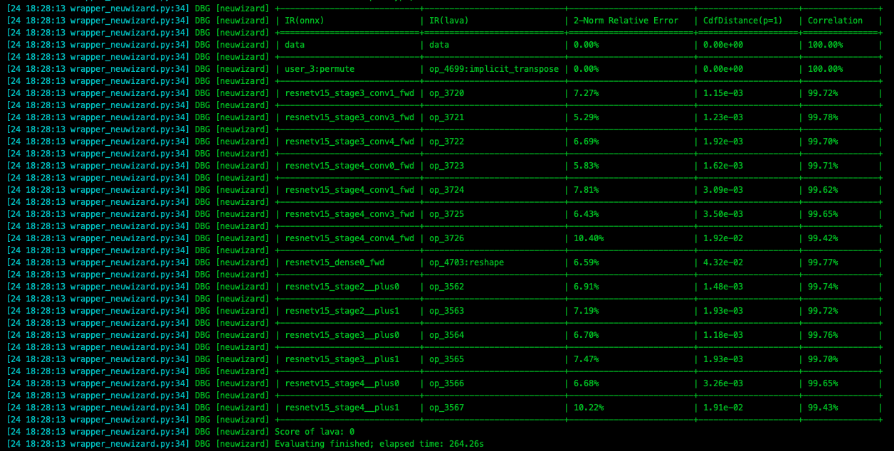
Warning

Note that adding this configuration will significantly increase the compilation time of the model.

5.6.3. Multiple inputs, different configurations for different channels CSC

CSC stands for Color Space Convert. The following configuration means that the data_0 input color space of the input model (i.e., the ONNX model) is BGR, The input color space of data_0 of the compiled output model (i.e., the JOINT model) will be modified to NV12, as described in tensor_conf configuration.

In short, it is what the input tensor is for the pre-compiled model, and what the input tensor is for the post-compiled model.

Code example 1

src_input_tensors {
  tensor_name: "data_0"
  color_space: TENSOR_COLOR_SPACE_BGR  # The color space of the `data_0` road input used to describe or illustrate the model
}
dst_input_tensors {
  tensor_name: "data_0"
  color_space: TENSOR_COLOR_SPACE_NV12  # Color space of the `data_0` road input used to modify the output model
}

where tensor_name is used to select a certain tensor. color_space is used to configure the color space of the current tensor.

Hint

The default value of color_space is TENSOR_COLOR_SPACE_AUTO , which is automatically recognized based on the number of channels entered by the model, 3-channel for BGR; 1-channel is GRAY . So if the color space is BGR, src_input_tensors can be left out, but sometimes src_input_tensors and dst_input_tensors usually come in pairs to better describe the information.

Code Example 2

src_input_tensors {
  color_space: TENSOR_COLOR_SPACE_AUTO
}
dst_input_tensors {
  color_space: TENSOR_COLOR_SPACE_AUTO
}

The number of channels is automatically selected based on the input tensor, which can be omitted but is not recommended.

Code Example 3

src_input_tensors {
tensor_name: "data_0"
  color_space: TENSOR_COLOR_SPACE_RGB # The color space of the original input model's `data_0` input is RGB
}
dst_input_tensors {
  tensor_name: "data_0"
  color_space: TENSOR_COLOR_SPACE_NV12
  color_standard: CSS_ITU_BT601_STUDIO_SWING
}

The above configuration means that the input color space of data_0 of the input model (i.e. ONNX model) is RGB, while the input color space of data_0 of the compiled output model (i.e. JOINT model) will be modified to NV12, and the color_standard will be configured as CSS_ITU_BT601_STUDIO_SWING .

5.6.4. cpu_lstm configuration

Hint

If there is an lstm structure in the model, you can configure it by referring to the following configuration file to ensure that the model will not have exceptions on this structure.

operator_conf_items {
  selector {}
  attributes {
    lstm_mode: LSTM_MODE_CPU
  }
}

A complete configuration file reference (containing cpu_lstm, rgb, nv12) example

input_type: INPUT_TYPE_ONNX
output_type: OUTPUT_TYPE_JOINT

src_input_tensors {
  tensor_name: "data"
  color_space: TENSOR_COLOR_SPACE_RGB
}
dst_input_tensors {
  tensor_name: "data"
  color_space: TENSOR_COLOR_SPACE_NV12
  color_standard: CSS_ITU_BT601_STUDIO_SWING
}

target_hardware: TARGET_HARDWARE_AX630 # You can override this configuration with command line arguments
neuwizard_conf {
  operator_conf {
    input_conf_items {
      attributes {
        input_modifications {
          input_normalization { # input data normalization, the order of mean/std is related to the color space of the input tensor
              mean: 0
              mean: 0
              mean: 0
              std: 255.0326
              std: 255.0326
              std: 255.0326
          }
        }
      }
    }
    operator_conf_items {  # lstm
      selector {}
      attributes {
        lstm_mode: LSTM_MODE_CPU
      }
    }
  }
  dataset_conf_calibration {
    path: "../imagenet-1k-images.tar"
    type: DATASET_TYPE_TAR
    size: 256
    batch_size: 32
  }
}
pulsar_conf {
  batch_size: 1
}

In the case of cpu_lstm only, the full configuration file is referenced below:

input_type: INPUT_TYPE_ONNX
output_type: OUTPUT_TYPE_JOINT
input_tensors {
  color_space: TENSOR_COLOR_SPACE_AUTO
}
output_tensors {
  color_space: TENSOR_COLOR_SPACE_AUTO
}
target_hardware: TARGET_HARDWARE_AX630
neuwizard_conf {
  operator_conf {
    input_conf_items {
      attributes {
        input_modifications {
          affine_preprocess {  # Affine the data, i.e. `* k + b`, to change the input data type of the compiled model
            slope: 1           # Change the input data type from floating point [0, 1) to uint8
            slope_divisor: 255
            bias: 0
          }
        }
      }
    }
    operator_conf_items {
      selector {}
      attributes {
        lstm_mode: LSTM_MODE_CPU
      }
    }
  }
  dataset_conf_calibration {
    path: "../imagenet-1k-images.tar"
    type: DATASET_TYPE_TAR
    size: 256
    batch_size: 32
  }
}
pulsar_conf {
  batch_size: 1
}

Hint

In attributes you can modify the data type directly, which is a forced type conversion, while affine in input_modifications converts floating-point data to UINT8 with a * k + b operation.

5.6.5. Dynamic Q values

Dynamic Q values are calculated automatically, and can be seen in the log message printed by run_joint.

Code example

dst_output_tensors {
  data_type: INT16
}

5.6.6. Static Q values

The difference between dynamic Q values is the explicit configuration of quantization_value.

Code example

dst_output_tensors {
  data_type: INT16
  quantization_value: 256
}

For a detailed description of the Q value see QValue Introduction

5.6.7. FLOAT input configuration

If you expect the compiled joint model of onnx to have the FLOAT32 type as input when you go to the board, you can configure prototxt according to the following example.

Code example

operator_conf {
  input_conf_items {
    attributes {
      type: FLOAT32   # Here it is agreed that the compiled model will have float32 as the input type
    }
  }
}

5.6.8. Multiple inputs, different data types for different channels

If you expect a two-way onnx compiled joint model to be loaded with UINT8 as input and FLOAT32 as input, See the following example prototxt configuration.

Code example

operator_conf {
  input_conf_items {
    selector {
      op_name: "input1"
    }
    attributes {
      type: UINT8
    }
  }
  input_conf_items {
    selector {
      op_name: "input2"
    }
    attributes {
      type: FLOAT32
    }
  }
}

5.6.9. 16bit quantization

Hint

Consider 16bit quantization when quantization accuracy is not sufficient.

Code example

operator_conf_items {
  selector {

  }
  attributes {
    input_feature_type: UINT16
    weight_type: INT8
  }
}

5.6.10. Joint Layout配置

Before toolchain axera/neuwizard:0.6.0.1, the output Layout of the toolchain compiled model varies depending on the situation and cannot be configured.

After 0.6.0.1, if the post-compile model output Layout is not configured in pulsar build or in the configuration options, the toolchain defaults to NCHW for the post-compile model output Layout.

Modify the joint output Layout via the configuration file as follows:

dst_output_tensors {
  tensor_layout: NHWC
}

Explicit configuration: add the --output_tensor_layout nhwc option to the pulsar build compiler directive.

Hint

Since the default layout layout of NHWC is internal to the hardware, it is recommended to use NHWC to get higher FPS.

5.6.11. Multiplex Calibration dataset

The following configuration describes a two-way input model with different calibration datasets for each way, where input0.tar and input1.tar are the data sets associated with the training dataset, respectively.

dataset_conf_calibration {
  dataset_conf_items {
    selector {
      op_name: "0"      # The tensor name of one input.
    }
    path: "input0.tar"  # Calibration dataset used `input0.tar`
  }
  dataset_conf_items {
    selector {
      op_name: "1"      # The tensor name of the other input.
    }
    path: "input1.tar"  # Calibration dataset used `input1.tar`
  }
  type: DATASET_TYPE_TAR
  size: 256
}

5.6.12. Calibration dataset as non-image type

For detection and classification models, the training data is generally a dataset of UINT8 images, For behavioral recognition models such as ST-GCN, the training data is generally a set of float type coordinate points. Currently, the Pulsar toolchain supports the configuration of calibration for non-image sets, which is described in the next section.

… attention:

- The ``calibration`` dataset should have the same distribution as the training and test datasets
- ``calibration`` should be given as a ``tar`` file consisting of ``.bin`` if it is not an image
- ``.bin`` must be consistent with the ``shape`` and ``dtype`` of the ``onnx`` model input

Take ST-GCN as an example of how to configure calibration for a non-image set.

ST-GCN Dual Input Example

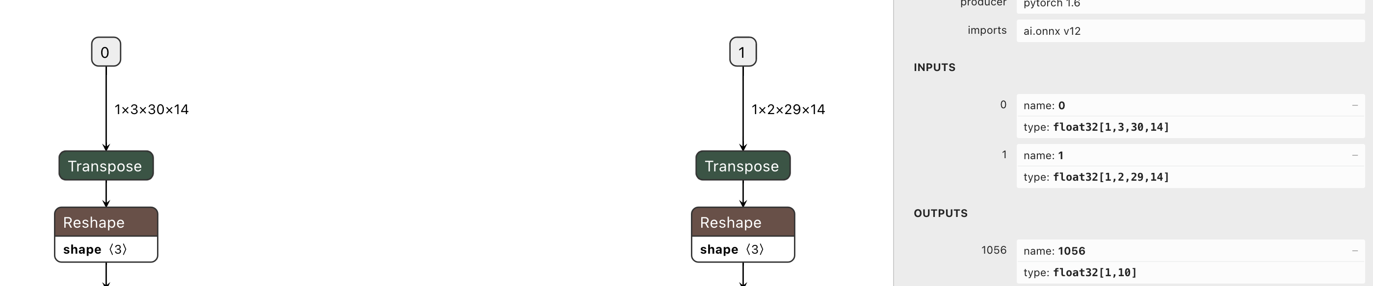
As you can see from the figure above:

• The input tensor_name of the two-way STGCN model is 0 and 1 respectively, and the dtype is float32.

• Following the :ref: multi_calibrations_input configuration method, it is easy to configure config correctly

• The details of how to create the tar file will be explained later

Dual input without pairing

The .tar file for calibration is explained in the case of a model with two inputs that does not require pairing.

Reference Code

import numpy as np
import os
import tarfile


def makeTar(outputTarName, sourceDir):
    # Create a tarball
    with tarfile.open( outputTarName, "w" ) as tar:
        tar.add(sourceDir, arcname=os.path.basename(sourceDir))

input_nums = 2 # two-way input, e.g. stgcn
case_nums = 100 # each tar contains 100 bin files

# Create bin files with numpy
for input_num in range(input_nums):
    for num in range(case_nums):
        if not os.path.exists(f "stgcn_tar_{input_num}"):
            os.makedirs(f "stgcn_tar_{input_num}")
        if input_num == 0:
            # input shape and dtype must be consistent with the input tensor of the original model
            # The input here is a random value, just as an example
            # The specific training or test dataset should be read in the real application
            input = np.random.rand(1, 3, 30, 14).astype(np.float32)
        elif input_num == 1:
            input = np.random.rand(1, 2, 29, 14).astype(np.float32)
        else:
            assert False
        input.tofile(f"./stgcn_tar_{input_num}/cnt_input_{input_num}_{num}.bin")

    # create tar file.
    makeTar(f"stgcn_tar_{input_num}.tar", f"./stgcn_tar_{input_num}" )

Configure the path of the tar file generated by the above script to dataset_conf_calibration.dataset_conf_items.path in config,

dual inputs need to be paired

• If dual inputs need to be paired, just make sure that the .bin files in both tar have the same name

• For example, cnt_input_0_0.bin, cnt_input_0_1.bin, … in stgcn_tar_0.tar. , cnt_input_0_n.bin , and the files in stgcn_tar_1.tar are named cnt_input_1_0.bin, cnt_input_1_1.bin, … , cnt_input_1_n.bin, the names of the files in the two tar are different, so it is not possible to pair the inputs

• In short, when you need to pair inputs with each other, the file names of the paired inputs should be the same

Hint

Note:

• Setting dtype is not supported for tofile.

• If you want to read in a bin file and restore the original data, you must specify dtype, and keep the same dtype as in tofile, otherwise you will get an error or a different number of elements.

• For example, if dtype is float64 at the time of tofile, and the number of elements is 1024, and float32 at the time of reading, then the number of elements will change to 2048, which is not as expected.

Code example is as follows:

input_0 = numpy.fromfile("./cnt_input_0_0.bin", dtype=np.float32)
input_0_reshape = input_0.reshape(1, 3, 30, 14)

When the dtype of the fromfile operation is different from the tofile, the reshape operation will report an error.

When calibration is a float set, you need to specify the dtype of the input tensor in the config, which is UINT8 by default. If this is not specified, a ZeroDivisionError may occur.

… attention:

For ``float`` inputs, note that the following is also required:

  .. code-block:: python
    :linenos:

    operator_conf {
      input_conf_items {
        attributes {
          type: FLOAT32
        }
      }
    }

5.6.13. Configuration dynamics batch

After setting dynamic batch, it supports any batch_size of not exceeding the maximum value during inference, which is more flexible to use:

pulsar_conf {
  batch_size_option: BSO_DYNAMIC # Make the compiled model support dynamic batch
  batch_size: 1
  batch_size: 2
  batch_size: 4 # Maximum batch_size is 4, requiring high performance for inference with batch_size of 1 2 or 4
}

5.6.14. Configure static batch

Compared to :ref:dynamic_batch_size <dynamic_batch_size>, static batch is simpler to configure, as follows:

pulsar_conf {
  batch_size: 8  # batch_size can be 8 or other value
}