4. 模型转换进阶指南
4.1. Pulsar Build 模型编译
本节介绍 pulsar build 命令完整使用方法.
4.1.1. 概述
pulsar build 用于模型优化、量化、编译等操作. 其运行示意图如下:
pulsar build 利用输入模型(model.onnx)和配置文件(config.prototxt), 编译得到输出模型(joint)和输出配置文件(output_config.prototxt).
pulsar build 的命令行参数将会覆盖配置文件中的某些对应部分, 并使 pulsar build 将覆盖过后得到的配置文件输出出来. 配置文件的详细介绍参见 配置文件详细说明.
pulsar build -h 可显示详细命令行参数:
 1root@xxx:/data# pulsar build -h
 2usage: pulsar build [-h] [--config CONFIG] [--output_config OUTPUT_CONFIG]
 3                    [--input INPUT [INPUT ...]] [--output OUTPUT [OUTPUT ...]]
 4                    [--calibration_batch_size CALIBRATION_BATCH_SIZE]
 5                    [--compile_batch_size COMPILE_BATCH_SIZE [COMPILE_BATCH_SIZE ...]]
 6                    [--batch_size_option {BSO_AUTO,BSO_STATIC,BSO_DYNAMIC}]
 7                    [--output_dir OUTPUT_DIR]
 8                    [--virtual_npu {0,311,312,221,222,111,112}]
 9                    [--input_tensor_color {auto,rgb,bgr,gray,nv12,nv21}]
10                    [--output_tensor_color {auto,rgb,bgr,gray,nv12,nv21}]
11                    [--output_tensor_layout {native,nchw,nhwc}]
12                    [--color_std {studio,full}]
13                    [--target_hardware {AX630,AX620,AX170}]
14                    [--enable_progress_bar]
15
16optional arguments:
17  -h, --help            show this help msesage and exit
18  --config CONFIG       .prototxt
19  --output_config OUTPUT_CONFIG
20  --input INPUT [INPUT ...]
21  --output OUTPUT [OUTPUT ...]
22  --calibration_batch_size CALIBRATION_BATCH_SIZE
23  --compile_batch_size COMPILE_BATCH_SIZE [COMPILE_BATCH_SIZE ...]
24  --batch_size_option {BSO_AUTO,BSO_STATIC,BSO_DYNAMIC}
25  --output_dir OUTPUT_DIR
26  --virtual_npu {0,311,312,221,222,111,112}
27  --input_tensor_color {auto,rgb,bgr,gray,nv12,nv21}
28  --output_tensor_color {auto,rgb,bgr,gray,nv12,nv21}
29  --output_tensor_layout {native,nchw,nhwc}
30  --color_std {studio,full}
31                        only support nv12/nv21 now
32  --target_hardware {AX630,AX620,AX170}
33                        target hardware to compile
34  --enable_progress_bar
提示
利用配置文件可以实现复杂功能, 而命令行参数只是起一个辅助作用. 另外, 命令行参数会 override 配置文件中的某些对应配置.
4.1.2. 参数详解
- pulsar build 参数解释
- --input
本次编译的输入模型路径, 对应
config.prototxt中的 input_path字段- --output
指定输出模型的文件名, 如
compiled.joint, 对应config.prototxt中的 output_path字段- --config
指定用于指导本次编译过程所用的基本配置文件. 如果为
pulsar build命令指定了命令行参数, 则转换模型过程中优先使用命令行参数中指定的值- --output_config
将本次编译过程所使用的完整配置信息输出到文件
- --target_hardware
指定编译输出模型所适用的硬件平台, 目前有
AX630和AX620可选- --virtual_npu
指定推理时使用的虚拟 NPU , 请根据
--target_hardware参数进行区别. 详情参见 芯片介绍 中的虚拟NPU部分- --output_dir
指定编译过程的工作目录. 默认为当前目录
- --calibration_batch_size
转模型过程中, 内部参数校准时所使用数据的
batch_size. 默认值为32- --batch_size_option
设置
joint格式模型所支持的batch类型:BSO_AUTO: 默认选项, 默认为静态batchBSO_STATIC: 静态batch, 推理时固定batch_size, 性能最优BSO_DYNAMIC: 动态batch, 推理时支持不超过最大值的任意batch_size, 使用最灵活
- --compile_batch_size
设置
joint格式模型所支持的batch size. 默认为1当指定了
--batch_size_option BSO_STATIC时,batch_size表示joint格式模型推理时能用的唯一batch size当指定了
--batch_size_option BSO_DYNAMIC时,batch_size表示joint格式模型推理时所能使用的最大batch size
- --input_tensor_color
指定 输入模型 的 输入数据 的色彩空间, 可选项:
- 默认选项:
auto, 根据模型输入 channel 数自动识别 3-channel 为
bgr1-channel 为
gray
- 默认选项:
其他可选项:
rgb,bgr,gray,nv12,nv21
- --output_tensor_color
指定 输出模型 的 输入数据 的色彩空间, 可选项:
- 默认选项:
auto, 根据模型输入 channel 数自动识别 3-channel 为
bgr1-channel 为
gray
- 默认选项:
其他可选项:
rgb,bgr,gray,nv12,nv21
- --color_std
指定用于在
RGB和YUV之间转换时所采用的转换标准, 可选项:legacy,studio和full, 默认值为legacy- --enable_progress_bar
编译时显示进度条. 默认不显示
- --output_tensor_layout
指定 输出 模型的 输出
tensor的layout, 可选:native: 默认选项, 历史遗留选项, 不推荐使用. 建议显式指定输出layoutnchwnhwc
注意
axera_neuwizard_v0.6.0.1及以后版本的工具链才支持此参数. 从axera_neuwizard_v0.6.0.1开始, 部分AX620A模型的输出tensor的默认layout可能与axera_neuwizard_v0.6.0.1之前版本的工具链编译出来的模型不同.AX630A模型的默认layout不受工具链版本的影响
代码示例
1pulsar build --input model.onnx --output compiled.joint --config my_config.prototxt --target_hardware AX620 --virtual_npu 111 --output_config my_output_config.prototxt
小技巧
当生成支持动态 batch 的 joint 模型时, 可以在 --compile_batch_size 后面指定多个常用的 batch_size, 以提高使用不超过这些值的 batch size 进行推理时的性能.
注意
指定多个 batch size 会增加 joint 模型文件的大小.
4.2. Pulsar Run 模型仿真与对分
本节介绍 pulsar run 命令完整使用方法.
4.2.1. 概述
pulsar run 用于在 x86 平台上对 joint 模型进行 x86仿真 和 精度对分.
pulsar run -h 可显示详细命令行参数:
 1root@xxx:/data# pulsar run -h
 2usage: pulsar run [-h] [--use_onnx_ir] [--input INPUT [INPUT ...]]
 3                  [--layer LAYER [LAYER ...]] [--output_gt OUTPUT_GT]
 4                  [--config CONFIG]
 5                  model [model ...]
 6
 7positional arguments:
 8  model
 9
10optional arguments:
11  -h, --help                   show this help msesage and exit
12  --use_onnx_ir                use NeuWizard IR for refernece onnx
13  --input INPUT [INPUT ...]    input paths or .json
14  --layer LAYER [LAYER ...]    input layer namse
15  --output_gt OUTPUT_GT        save gt data in dir
16  --config CONFIG
- pulsar run 参数解释
必要参数
model.jointmodel.onnx- --input
可以指定多个输入数据, 并作为仿真
inference的输入数据. 支持jpg、png、bin等格式, 需要保证其个数与模型输入层个数一致- --layer
- 不是必需项当模型有多路输入时, 用于指定输入数据对应哪一层. 其顺序与
--input呈对照关系比如--input file1.bin file2.bin --layer layerA layerB就代表给layerA输入file1.bin、给layerB输入file2.bin, 需要保证--layer的长度与--input的长度一致 - --use_onnx_ir
- 当使用
onnx格式模型作为对分参考模型时, 此选项用以告诉pulsar run在内部用NeuWizard IR推理onnx模型. 默认不使用NeuWizard IR此选项只有在指定了--onnx时才有意义, 该选项可忽略 - --output_gt
指定用于存放目标模型的仿真
inference结果和上板输入数据的目录. 默认不输出- --config
指定配置文件, 用于指导
pulsar run在内部转换参考模型. 一般使用pulsar build的--output_config选项输出的配置文件
pulsar run 代码示例
pulsar run model.onnx compiled.joint --input test.jpg --config my_output_config.prototxt --output_gt gt
4.3. Pulsar Info 查看模型信息
注意
注意: 只有在版本号大于 0.6.1.2 的 docker 工具链中才能正常使用 pulsar info 功能.
对于旧版本工具链转出的 .joint 模型, 无法通过 pulsar info 查看正确的信息, 需要利用新版本工具链重新转换. 原因在于旧版本 joint 中的 Performance.txt 文件不包含 onnx layer name 信息, 需要重新转换生成.
pulsar info 用于查看 onnx 和 joint 模型的信息, 并支持将模型信息保存为 html, grid, jira 等格式.
用法命令
pulsar info model.onnx/model.joint
参数列表
$ pulsar info -h

usage: pulsar info [-h] [--output OUTPUT] [--output_json OUTPUT_JSON]
                  [--layer_mapping] [--performance] [--part_info]
                  [--tablefmt TABLEFMT]
                  model

positional arguments:
  model

optional arguments:
  -h, --help            show this help msesage and exit
  --output OUTPUT       path to output dir
  --output_json OUTPUT_JSON
  --layer_mapping
  --performance
  --part_info
  --tablefmt TABLEFMT   possible formats (html, grid, jira, etc.)
参数说明
- pulsar info 参数解释
- --output
指定模型信息保存目录, 默认不保存
- --output_json
以 Json 形式保存模型的完整信息, 默认不保存
- --layer_mapping
显示 Joint 模型的 layer_mapping 信息, 默认不显示
可以用于查看 onnx layer 与转换后的 lava layer 间的对应关系
- --performance
显示 Joint 模型的 performance 信息, 默认不显示
- --part
显示 Joint 模型每个部分的全部信息, 默认不显示
- --tablefmt
- 指定模型信息显示和保存格式, 可选项:
simple: 默认选择项
grid
html
jira
… 任意 tabulate 库支持的 tablefmt 格式
示例: 查看模型基本信息
pulsar info resnet18.joint

# output log
[24 18:40:10 wrapper_pulsar_info.py:32] Information of resnet18.joint:
IO Meta Info:
NAME                  I/O?    SHAPE             DTYPE    LAYOUT
--------------------  ------  ----------------  -------  --------
data                  INPUT   [1, 224, 224, 3]  uint8    NHWC
resnetv15_dense0_fwd  OUTPUT  [1, 1000]         float32  NCHW

Approx System Memory: 13.84 MB
Approx Standard Memory: 0 B
Approx Memory: 13.84 MB

Virtual NPU: AX620_VNPU_111
Static Batch: 1
Toolchain Version: dfdce086b
示例: 查看 onnx layer 与编译后模型的 layer 之间的对应关系
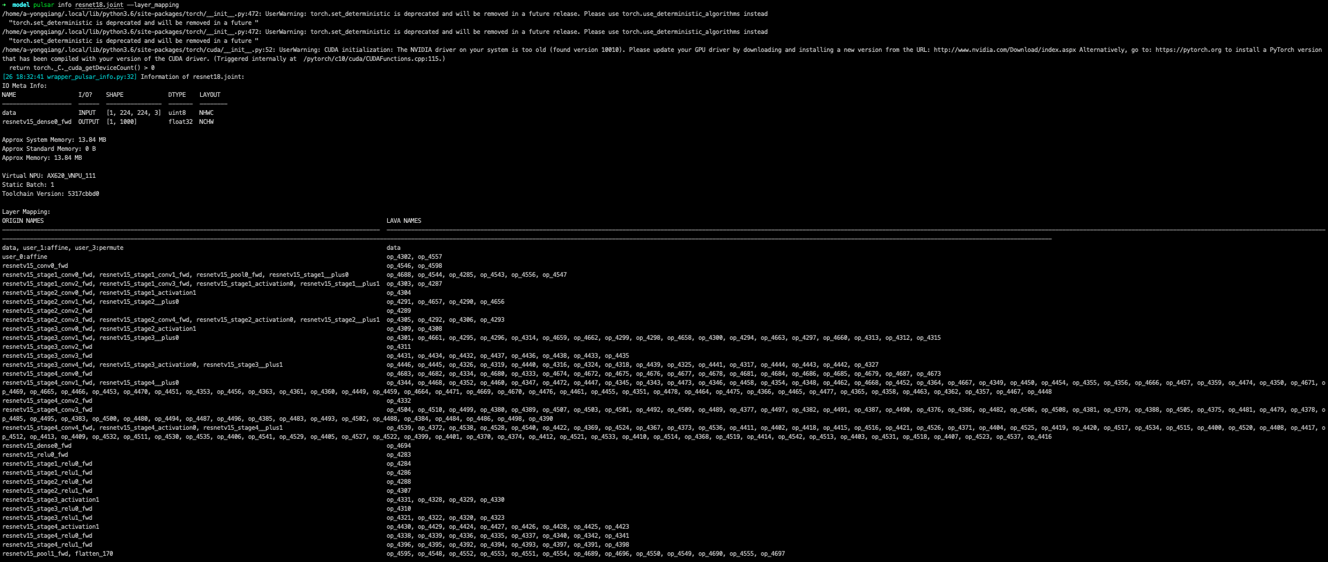
其中 ORIGIN_NAmse 为原 onnx 的 layer name, 而 LAVA_NAmse 则为编译后模型的 layer name.
备注
在 pulsar info 中指定参数:
--layer_mapping参数可查看onnx_layer_name与转换后模型layer_name之间的对应关系--performance参数可以查看各个layer的performance信息
4.4. Pulsar Version 查看工具链版本
pulsar version 用于获取工具的版本信息.
提示
如果需要向我们提供工具链的错误信息, 请将您所使用的工具链版本信息一并提交给我们.
代码示例
pulsar version
示例结果
0.5.34.2
7ca3b9d5
4.5. 配套工具
Pulsar 工具链还提供了其他常用的网络模型处理工具, 有助于使用者对网络模型进行格式转换等功能.
4.5.1. Caffe2ONNX
在 Pulsar 的 Docker 镜像中预装了 dump_onnx.sh 工具, 提供将 Caffe 模型转换成 ONNX 模型的功能, 从而间接拓展了 pulsar build 对 Caffe 模型的支持. 具体使用方法如下所示:
dump_onnx.sh -h 可显示详细命令行参数:
1root@xxx:/data$ dump_onnx.sh
2Usage: /root/caffe2onnx/dump_onnx.sh [prototxt] [caffemodel] [onnxfile]
选项解释
[prototxt]
输入的
caffe模型的*.prototxt文件路径[caffemodel]
输入的
caffe模型的*.caffemodel文件路径[onnxfile]
输出的
*.onnx模型文件路径
代码示例
1root@xxx:/data$ dump_onnx.sh model/mobilenet.prototxt model/mobilenet.caffemodel model/mobilenet.onnx
log 信息示例如下
 1root@xxx:/data$ dump_onnx.sh model/mobilenet.prototxt model/mobilenet.caffemodel model/mobilenet.onnx
 22. start model conversion
 3=================================================================
 4Converting layer: conv1 | Convolution
 5Input:  ['data']
 6Output:  ['conv1']
 7=================================================================
 8Converting layer: conv1/bn | BatchNorm
 9Input:  ['conv1']
10Output:  ['conv1']
11=================================================================
12Converting layer: conv1/scale | Scale
13Input:  ['conv1']
14Output:  ['conv1']
15=================================================================
16Converting layer: relu1 | ReLU
17Input:  ['conv1']
18Output:  ['conv1']
19=================================================================
20####省略若干行 ############
21=================================================================
22Node:  prob
23OP Type:  Softmax
24Input:  ['fc7']
25Output:  ['prob']
26====================================================================
272. onnx model conversion done
284. save onnx model
29model saved as: model/mobilenet.onnx
4.5.2. parse_nw_model
功能
统计 joint 模型 cmm 使用情况
1usage: parse_nw_model.py [-h] [--model MODEL]
2
3optional arguments:
4  -h, --help     show this help msesage and exit
5  --model MODEL  dot_neu or joint file
使用方法示例
以下命令只适用于工具链 docker 环境
1python3 /root/python_modules/super_pulsar/super_pulsar/tools/parse_nw_model.py --model yolox_l.joint
2python3 /root/python_modules/super_pulsar/super_pulsar/tools/parse_nw_model.py --model part_0.neu
返回结果示例
1{'McodeSize': 90816, 'WeightsNum': 1, 'WeightsSize': 568320, 'ringbuffer_size': 0, 'input_num': 1, 'input_size': 24576, 'output_num': 16, 'output_size': 576}
字段说明
字段 |
说明 |
|---|---|
单位 |
Byte |
McodeSize |
二进制代码 Size |
WeightsNum |
表示权重个数 |
WeightsSize |
权重 Size |
ringbuffer_size |
表示模型运行期间需要申请的 DDR Swap 空间 |
input_num |
表示模型的输入 Tensor 数 |
input_size |
输入 Tensor Size |
output_num |
输出 Tensor 数 |
output_size |
输出 Tensor Size |
提示
该脚本统计 joint 模型中所有 .neu 的 CMM 内存, 返回结果为所有 .neu 文件的解析结果之和.
4.5.3. joint 模型初始化速度补丁工具
概述
提示
对于 neuwizard-0.5.29.9 及更早版本工具链转换的 joint 模型文件,
可以使用 optimize_joint_init_time.py 工具离线刷新, 以减少 joint 模型加载时间, 推理结果和时间不变.
使用方法
cd /root/python_modules/super_pulsar/super_pulsar/tools
python3 optimize_joint_init_time.py --input old.joint --output new.joint
4.5.4. 将 joint 模型中的 ONNX 子图转为 AXEngine 子图
使用方法
提示
如下一条指令即可将名为 input.joint 的 joint 模型(以 ONNX 作为 CPU 后端实现)转为 joint 模型(以 AXEngine 作为 CPU 后端实现), 并且开启优化模式.
python3 /root/python_modules/super_pulsar/super_pulsar/tools/joint_onnx_to_axe.py --input input.joint --output output.joint --optimize_slim_model
参数释义
- 参数释义
- --input
转换工具的输入
joint模型路径- --output
转换工具的输出
joint模型路径- --optimize_slim_model
开启优化模式. 当网络输出特征图较小时建议开启, 否则不建议
4.5.5. wbt_tool 使用说明
背景
某些模型在不同使用场景下需要不同的网络权重, 例如 VD 模型的使用场景分为白天和夜晚, 两个网络结构一样, 但权重不一样, 是否可以设置成不同场景使用不同的权重, 即同一个模型保存多组权重信息
可以通过
Pulsar工具链Docker中提供的wbt_tool脚本可以实现一个模型, 多套参数的需求
工具概述
工具路径: /root/python_modules/super_pulsar/super_pulsar/tools/wbt_tool.py, 注意需要给 wbt_tool.py 可执行权限
# 添加可执行权限
chmod a+x /root/python_modules/super_pulsar/super_pulsar/tools/wbt_tool.py
- wbt_tool 功能参数
- info
查看操作, 可以查看
joint模型的wbt名称信息, 如果是None, 在fuse时需要手动指定- fuse
合并操作, 将多个网络结构一样, 网络权重不同的
joint模型, 合成一个具有多份权重的joint模型- split
拆分操作, 将一个具有多份权重的
joint模型, 拆分成多个网络结构一样, 网络权重不同的joint模型
使用限制
警告
不支持含多份 wbt 的 joint 模型之间的合并,
有需求时请先拆分成多个含单份 wbt 的 joint 模型, 再和其他模型合并.
示例1
查看模型 model.joint 的 wbt 信息:
<wbt_tool> info model.joint

part_0.neu's wbt_namse:
    index 0: wbt_#0
    index 1: wbt_#1
提示
其中 <wbt_tool> 为 /root/python_modules/super_pulsar/super_pulsar/tools/wbt_tool.py
示例2
合并名为 model1.joint, model2.joint 的两个模型至名为 model.joint 的模型, 使用 joint 模型中自带的 wbt_name
<wbt_tool> fuse --input model1.joint model2.joint --output model.joint
注意
如果 wbt_tool info 查看到 joint 模型的 wbt_name 为 None, 需要手动指定 wbt_name, 否则 fuse 时会报错.
示例3
拆分名为 model.joint 的模型至两个名为 model1.joint, model2.joint 的模型
<wbt_tool> split --input model.joint --output model1.joint model2.joint
示例4
合并名为 model1.joint, model2.joint 的两个模型至名为 model.joint 的模型, 且规定 model1.joint 模型中的 wbt_name 为 wbt1, wbt2, model2.joint 模型中的 wbt_name 为 wbt2
<wbt_tool> fuse --input model1.joint model2.joint --output model.joint --wbt_name wbt1 wbt2
示例5
拆分名为 model.joint 的模型, 该模型有四个 wbt 参数, index 为 0, 1, 2, 3,
只取 index 为 1, 3 的那两个 wbt, 包装为 joint 模型, 并取名为 model_idx1.joint, model_idx3.joint
<wbt_tool> split --input model.joint --output model_idx1.joint model_idx3.joint --indexes 1 3
注意
如果有使用上的问题, 请联系相关 FAE 同学进行支持.
4.6. 不同场景下的 config prototxt 配置方法
提示
Pulsar 通过合理配置 config 可以完成复杂的功能, 下面对一些常见场景下 config 配置进行说明.
注意: 本节所提供的代码示例均为代码片段, 需要用户手动添加到合适的位置.
4.6.1. 搜索 PTQ 模型混合比特配置
前置工作
确保当前的 onnx 模型和配置文件 config_origin.prototxt 在 pulsar build 时可以成功转换为 joint 模型.
复制并修改配置文件
COPY 配置文件 config_origin.prototxt 并将其命名为 mixbit.prototxt, 然后对 mixbit.prototxt 作如下修改:
output_type指定为OUTPUT_TYPE_SUPERNET在
neuwizard_conf内添加task_conf并按需添加混合比特搜索相关配置
config 示例如下:
 1# 基本配置参数: 输入输出
 2...
 3output_type: OUTPUT_TYPE_SUPERNET
 4...
 5
 6# neuwizard 工具的配置参数
 7neuwizard_conf {
 8    ...
 9    task_conf{
10      task_strategy: TASK_STRATEGY_SUPERNET # 不可修改
11      supernet_options{
12        strategy: SUPERNET_STRATEGY_MIXBIT # 不可修改
13        mixbit_params{
14          target_w_bit: 8 # 设置平均 weight bit, 支持小数但数值必须在 w_bit_choices 的区间内
15          target_a_bit: 6 # 设置平均 feature bit, 支持小数但数值必须在 f_bit_choices 的区间内
16          w_bit_choices: 8 # weight 比特目前仅支持 [4, 8], 由于 prototxt 的限制必须分行写各个选项
17          a_bit_choices: 4 # feature 比特目前仅支持 [4, 8, 16], 由于 prototxt 的限制必须分行写各个选项
18          a_bit_choices: 8
19          # 目前支持 MIXBIT_METRIC_TYPE_HAWQv2, MIXBIT_METRIC_TYPE_MSE, MIXBIT_METRIC_TYPE_COS_SIM 三种,
20          # 其中 hawqv2 速度较慢且可能需要开小 calibration batchsize, 推荐使用 MIXBIT_METRIC_TYPE_MSE
21          metric_type: MIXBIT_METRIC_TYPE_MSE
22        }
23      }
24    }
25  ...
26}
注意
目前 metric_type 支持配置
MIXBIT_METRIC_TYPE_HAWQv2
MIXBIT_METRIC_TYPE_MSE
MIXBIT_METRIC_TYPE_COS_SIM
三种, 其中 HAWQv2 速度较慢且可能需要开小 calibration batchsize, 推荐使用 MIXBIT_METRIC_TYPE_MSE.
进行 mixbit 搜索
在工具链 docker 中执行如下命令
1pulsar build --config mixbit.prototxt --input your.onnx # 如果模型路径已经配置在 config 中, 可省略 --input xxx
编译结束后会在当前目录产生 mixbit_operator_config.prototxt 文件和 onnx_op_bits.txt 文件.
mixbit_operator_config.prototxt是可直接用于配置prototxt的混合比特搜索结果onnx_op_bits.txt中输出了.onnx模型中各权重层的输入feature和weight bit, 以及各bit的sensitivity计算结果 (数值越小表明对模型表现影响越小)
注意
在搜 mixbit 时, mixbit.prototxt 中如果配置了 evaluation_conf 域, 编译过程中会报错, 但是不影响最终的输出结果, 因此可以忽略.
将 mixbit 搜索结果添加至配置文件, 编译出基于 mixbit 配置的模型.
将 mixbit_operator_config.prototxt 中的所有内容直接复制到 config_origin.prototxt (不包含上述混合比特相关配置) 文件中的 neuwizard_conf->operator_conf 内, 示例如下:
 1# neuwizard 工具的配置参数
 2neuwizard_conf {
 3    ...
 4    operator_conf{
 5      ...
 6      operator_conf_items {
 7          selector {
 8              op_name: "192"
 9          }
10          attributes {
11              input_feature_type: UINT4
12              weight_type: INT8
13          }
14      }
15      operator_conf_items {
16          selector {
17              op_name: "195"
18          }
19          attributes {
20              input_feature_type: UINT8
21              weight_type: INT4
22          }
23      }
24      ...
25  }
26  ...
27}
在工具链 docker 中执行如下命令:
1# 命令的参数需要根据实际需求配置, 这里仅用于说明问题
2pulsar build --config config_origin.prototxt --input your.onnx
最后得到编译后的混合比特模型 your.joint. 以下分别测试了 Resnet18 和 Mobilenetv2 在配置不同比特时模型的表现情况.
Resnet18
resnet18 |
Float top1 |
QPS |
search time |
|---|---|---|---|
float |
69.88% |
/ |
/ |
8w8f |
69.86% |
92.92 |
/ |
[mse or cos_sim] 6w8f |
68.58% |
135.39 |
4s |
hawqv2 6w8f |
68.58% |
135.39 |
3min |
[mse or cos_sim] 5w8f |
66.52% |
153.14 |
4s |
hawqv2 5w8f |
66.52% |
153.14 |
3min |
hawqv2 5w7f |
65.72% |
157.59 |
7min |
[mse or cos_sim] 5w7f |
65.8% |
157.35 |
8s |
4w8f |
55.66% |
169.35 |
/ |
Mobilenetv2
mobilenetv2 |
float top1 |
QPS |
search time |
|---|---|---|---|
float |
72.3% |
/ |
/ |
8w8f |
71.02% |
165.78 |
/ |
hawqv2 6w8f |
68.96% |
172.10 |
61min |
[mse or cos_sim] 6w8f |
69.2% |
173.33 |
6s |
[mse or cos_sim] 8w6f |
69.56% |
174.30 |
4s |
备注
上述繁琐的操作本质上是将搜索出的结果配置到 config_origin.prototxt 中, 基于搜索的配置编译出 joint 模型.
4.6.2. 逐层对分
注意
注意: 只有在版本号大于 0.6.1.2 的 docker 工具链中才能正常使用逐层对分功能.
需要在配置文件中加入以下内容
dataset_conf_error_measurement {
      path: "../dataset/imagenet-1k-images.tar"
      type: DATASET_TYPE_TAR         # 数据集类型为 tar package
      size: 256                      # 量化校准过程中实际使用的图片张数
 }

 evaluation_conf {
      path: "neuwizard.evaluator.error_measure_evaluator"
      type: EVALUATION_TYPE_ERROR_MEASURE
      source_ir_types: IR_TYPE_ONNX
      ir_types: IR_TYPE_LAVA
      score_compare_per_layer: true
 }
完整示例如下(以 resnet18 config 为例)
# 基本配置参数:输入输出
input_type: INPUT_TYPE_ONNX
output_type: OUTPUT_TYPE_JOINT

# 硬件平台选择
target_hardware: TARGET_HARDWARE_AX620

# CPU 后端选择,默认采用 AXE
cpu_backend_settings {
    onnx_setting {
        mode: DISABLED
    }
    axe_setting {
        mode: ENABLED
        axe_param {
            optimize_slim_model: true
        }
    }
}

# 模型输入数据类型设置
src_input_tensors {
    color_space: TENSOR_COLOR_SPACE_RGB
}

dst_input_tensors {
    color_space: TENSOR_COLOR_SPACE_RGB
    # color_space: TENSOR_COLOR_SPACE_NV12  # 若输入数据是 NV12, 则使用该配置
}

# neuwizard 工具的配置参数
neuwizard_conf {
    operator_conf {
        input_conf_items {
            attributes {
                input_modifications {
                    affine_preprocess {
                        slope: 1
                        slope_divisor: 255
                        bias: 0
                    }
                }
                input_modifications {
                    input_normalization {
                        mean: [0.485,0.456,0.406]  ## 均值
                        std: [0.229,0.224,0.255]   ## 方差
                    }
                }
            }
        }
    }
    dataset_conf_calibration {
        path: "../dataset/imagenet-1k-images.tar" # 设置 PTQ 校准数据集路径
        type: DATASET_TYPE_TAR         # 数据集类型:tar 包
        size: 256                      # 量化校准过程中实际使用的图片张数
        batch_size: 1
    }

    dataset_conf_error_measurement {
        path: "../dataset/imagenet-1k-images.tar"
        type: DATASET_TYPE_TAR         # 数据集类型: tar 包
        size: 4                        # 逐层对分过程中实际使用的图片张数
    }

    evaluation_conf {
        path: "neuwizard.evaluator.error_measure_evaluator"
        type: EVALUATION_TYPE_ERROR_MEASURE
        source_ir_types: IR_TYPE_ONNX
        ir_types: IR_TYPE_LAVA
        score_compare_per_layer: true
    }
}

# 输出 layout 设置, 建议使用 NHWC, 速度更快
dst_output_tensors {
    tensor_layout:NHWC
}

# pulsar compiler 的配置参数
pulsar_conf {
    ax620_virtual_npu: AX620_VIRTUAL_NPU_MODE_111   # 业务场景需要使用 ISP, 则必须使用 vNPU 111 配置, 1.8Tops 算力给用户的算法模型
    batch_size: 1
    debug : false
}
在 pulsar build 过程中, 会打印出模型每一层的精度损失情况, 如下图所示.
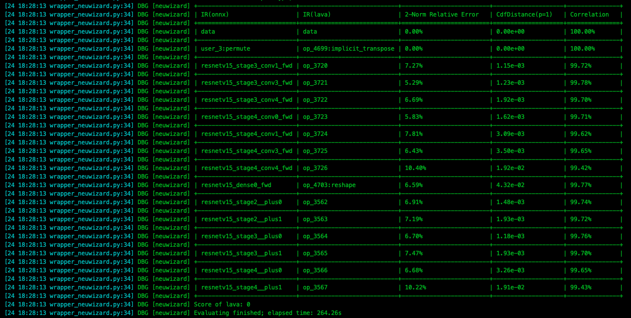
警告
注意, 添加此配置后会大幅度增加模型的编译时间.
4.6.3. 多路输入, 不同路配置不同 CSC
CSC 为色彩空间转换 (Color Space Convert) 的缩写. 以下配置表示输入模型(即 ONNX 模型)的 data_0 输入色彩空间为 BGR,
而编译后的输出模型(即 JOINT 模型)的 data_0 的输入色彩空间将被修改为 NV12, 详细信息可以参考 tensor_conf配置.
简而言之, 就是编译前的模型, 输入 tensor 是什么属性, 而编译后的模型, 输入 tensor 又是什么属性.
代码示例1
1src_input_tensors {
2  tensor_name: "data_0"
3  color_space: TENSOR_COLOR_SPACE_BGR  # 用于描述或说明模型的 `data_0` 路输入的色彩空间
4}
5dst_input_tensors {
6  tensor_name: "data_0"
7  color_space: TENSOR_COLOR_SPACE_NV12  # 用于修改输出模型的 `data_0` 路输入的色彩空间
8}
其中 tensor_name 用于选择某一路 tensor . color_space 用于配置当前 tensor 的色彩空间.
提示
color_space 的默认值为 TENSOR_COLOR_SPACE_AUTO , 会根据模型输入 channel 数自动识别, 3-channel 为 BGR;
1-channel 为 GRAY . 所以如果色彩空间为 BGR 时, 可以不配置 src_input_tensors , 但是有时候为了更好地描述信息, src_input_tensors 和 dst_input_tensors 通常会成对出现.
代码示例2
1src_input_tensors {
2  color_space: TENSOR_COLOR_SPACE_AUTO
3}
4dst_input_tensors {
5  color_space: TENSOR_COLOR_SPACE_AUTO
6}
根据输入 tensor 的 channel 数自动选择, 此配置项可省略, 但不推荐.
代码示例3
1src_input_tensors {
2tensor_name: "data_0"
3  color_space: TENSOR_COLOR_SPACE_RGB  # 原始输入模型的 `data_0` 输入的色彩空间是 RGB
4}
5dst_input_tensors {
6  tensor_name: "data_0"
7  color_space: TENSOR_COLOR_SPACE_NV12
8  color_standard: CSS_ITU_BT601_STUDIO_SWING
9}
以上配置表示输入模型(即 ONNX 模型)的 data_0 输入色彩空间为 RGB, 而编译后的输出模型(即 JOINT 模型)的 data_0 的输入色彩空间将被修改为 NV12, 同时将 color_standard 配置为 CSS_ITU_BT601_STUDIO_SWING .
4.6.4. cpu_lstm 配置
提示
如果模型中存在 lstm 结构, 可以参考如下配置文件进行配置, 保证模型在此结构上不会出现异常.
1operator_conf_items {
2  selector {}
3  attributes {
4    lstm_mode: LSTM_MODE_CPU
5  }
6}
一个完整的配置文件参考(包含 cpu_lstm, rgb, nv12)示例
 1input_type: INPUT_TYPE_ONNX
 2output_type: OUTPUT_TYPE_JOINT
 3
 4src_input_tensors {
 5  tensor_name: "data"
 6  color_space: TENSOR_COLOR_SPACE_RGB
 7}
 8dst_input_tensors {
 9  tensor_name: "data"
10  color_space: TENSOR_COLOR_SPACE_NV12
11  color_standard: CSS_ITU_BT601_STUDIO_SWING
12}
13
14target_hardware: TARGET_HARDWARE_AX630  # 可以使用命令行参数覆盖此配置
15neuwizard_conf {
16  operator_conf {
17    input_conf_items {
18      attributes {
19        input_modifications {
20          input_normalization {  # 输入数据归一化, mean/std 的顺序与输入 tensor 的色彩空间有关
21              mean: 0
22              mean: 0
23              mean: 0
24              std: 255.0326
25              std: 255.0326
26              std: 255.0326
27          }
28        }
29      }
30    }
31    operator_conf_items {  # lstm
32      selector {}
33      attributes {
34        lstm_mode: LSTM_MODE_CPU
35      }
36    }
37  }
38  dataset_conf_calibration {
39    path: "../imagenet-1k-images.tar"
40    type: DATASET_TYPE_TAR
41    size: 256
42    batch_size: 32
43  }
44}
45pulsar_conf {
46  batch_size: 1
47}
只有 cpu_lstm 的情况下, 完整配置文件参考如下:
 1input_type: INPUT_TYPE_ONNX
 2output_type: OUTPUT_TYPE_JOINT
 3input_tensors {
 4  color_space: TENSOR_COLOR_SPACE_AUTO
 5}
 6output_tensors {
 7  color_space: TENSOR_COLOR_SPACE_AUTO
 8}
 9target_hardware: TARGET_HARDWARE_AX630
10neuwizard_conf {
11  operator_conf {
12    input_conf_items {
13      attributes {
14        input_modifications {
15          affine_preprocess {  # 对数据做 affine 操作, 即 `* k + b` , 用于改变编译后模型的输入数据类型
16            slope: 1           # 即将输入数据类型由浮点数 [0, 1) 类型修改为 uint8
17            slope_divisor: 255
18            bias: 0
19          }
20        }
21      }
22    }
23    operator_conf_items {
24      selector {}
25      attributes {
26        lstm_mode: LSTM_MODE_CPU
27      }
28    }
29  }
30  dataset_conf_calibration {
31    path: "../imagenet-1k-images.tar"
32    type: DATASET_TYPE_TAR
33    size: 256
34    batch_size: 32
35  }
36}
37pulsar_conf {
38  batch_size: 1
39}
提示
在 attributes 可以直接修改数据类型, 属于 强制类型转换 , 而 input_modifications 中的 affine 将浮点类型的数据转换为 UINT8 时, 会有 * k + b 操作.
4.6.5. 动态 Q 值
动态 Q 值会被自动计算, 可以通过 run_joint 打印的log信息查看具体值.
代码示例
1dst_output_tensors {
2  data_type: INT16
3}
4.6.6. 静态 Q 值
与动态 Q 值的区别在于显式配置 quantization_value.
代码示例
1dst_output_tensors {
2  data_type: INT16
3  quantization_value: 256
4}
关于 Q 值的详细描述参见 Q值介绍
4.6.7. FLOAT 输入配置
如果期望 onnx 编译后的 joint 模型, 能在上板时以 FLOAT32 类型作为输入,
可以按照以下示例对 prototxt 配置.
代码示例
1operator_conf {
2  input_conf_items {
3    attributes {
4      type: FLOAT32   # 这里约定了编译后的模型以 float32 作为输入类型
5    }
6  }
7}
4.6.8. 多路输入, 不同路设置不同的数据类型
如果期望双路 onnx 编译后的 joint 模型, 能在上板时一路以 UINT8 为输入, 另一路以 FLOAT32 为输入,
可以参考以下示例 prototxt 配置.
代码示例
 1operator_conf {
 2  input_conf_items {
 3    selector {
 4      op_name: "input1"
 5    }
 6    attributes {
 7      type: UINT8
 8    }
 9  }
10  input_conf_items {
11    selector {
12      op_name: "input2"
13    }
14    attributes {
15      type: FLOAT32
16    }
17  }
18}
4.6.9. 16bit 量化
提示
在量化精度不足时, 可以考虑 16bit 量化.
代码示例
1operator_conf_items {
2  selector {
3
4  }
5  attributes {
6    input_feature_type: UINT16
7    weight_type: INT8
8  }
9}
4.6.10. Joint Layout配置
在工具链 axera/neuwizard:0.6.0.1 之前, 工具链编译后模型的输出 Layout 根据情况而异, 无法配置.
在 0.6.0.1 版本之后, 如果不在 pulsar build 或者配置选项中配置编译后模型输出 Layout, 则工具链默认设置编译后模型输出 Layout 为 NCHW.
通过配置文件修改 joint 输出 Layout 参考如下:
1dst_output_tensors {
2  tensor_layout: NHWC
3}
显式配置方式为: 在 pulsar build 编译指令中添加 --output_tensor_layout nhwc 选项.
提示
由于硬件内部是默认 NHWC 的 layout 排布, 因此更推荐使用 NHWC 以获得更高的 FPS.
4.6.11. 多路 Calibration 数据集
如下配置描述了双路输入模型中每一路采用不同 calibration 数据集的情况, 其中 input0.tar 与 input1.tar 分别是与训练数据集相关的数据集合.
 1dataset_conf_calibration {
 2  dataset_conf_items {
 3    selector {
 4      op_name: "0"      # 一路输入的 tensor name.
 5    }
 6    path: "input0.tar"  # 使用的校准数据集 `input0.tar`
 7  }
 8  dataset_conf_items {
 9    selector {
10      op_name: "1"      # 另一路输入的 tensor name.
11    }
12    path: "input1.tar"  # 使用的校准数据集 `input1.tar`
13  }
14  type: DATASET_TYPE_TAR
15  size: 256
16}
4.6.12. Calibration 数据集为非图像类型
对于检测和分类模型, 训练数据一般为 UINT8 图像组成的数据集,
而对于诸如 ST-GCN 等行为识别模型, 其训练数据一般为 float 类型的坐标点构成的集合.
目前 Pulsar 工具链支持配置非图像集的 calibration, 接下来对具体配置方法进行说明.
注意
calibration数据集应与训练数据集和测试数据集具有相同的分布calibration为非图像的情况下需要给出由.bin组成的tar文件.bin必须保证与onnx模型输入的shape和dtype一致
以 ST-GCN 为例, 说明如何配置非图像集的 calibration.
ST-GCN双路输入示例
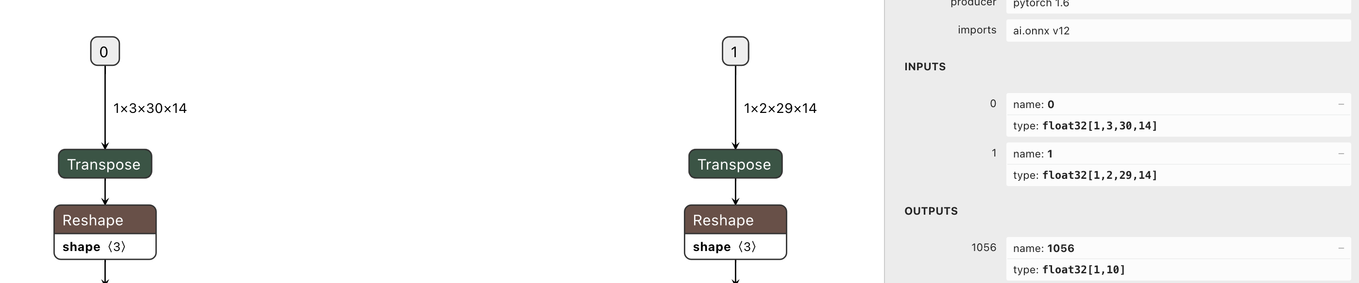
从上图可知:
双路
STGCN模型的输入tensor_name分别为0和1,dtype为float32按照 多路 calibration 的配置方法, 可以很容易地将
config配置正确
tar文件的具体制作方式, 将在后文中说明
双路输入但不需要配对
在模型双路输入不需要配对的情况下, 说明如何制作 calibration 的 .tar 文件.
参考代码
 1import numpy as np
 2import os
 3import tarfile
 4
 5
 6def makeTar(outputTarName, sourceDir):
 7    # 打 tar 包
 8    with tarfile.open( outputTarName, "w" ) as tar:
 9        tar.add(sourceDir, arcname=os.path.basename(sourceDir))
10
11input_nums = 2   # 双路输入, 如 stgcn
12case_nums = 100  # 每个 tar 中包含 100 个 bin 文件
13
14# 通过 numpy 创建 bin 文件
15for input_num in range(input_nums):
16    for num in range(case_nums):
17        if not os.path.exists(f"stgcn_tar_{input_num}"):
18            os.makedirs(f"stgcn_tar_{input_num}")
19        if input_num == 0:
20            # 输入 shape 和 dtype 必须和原始模型的输入 tensor 保持一致
21            # 这里的 input 是一个随机值, 仅仅作为一个 example
22            # 在实际应用中应读取具体的训练或测试数据集
23            input = np.random.rand(1, 3, 30, 14).astype(np.float32)
24        elif input_num == 1:
25            input = np.random.rand(1, 2, 29, 14).astype(np.float32)
26        else:
27            assert False
28        input.tofile(f"./stgcn_tar_{input_num}/cnt_input_{input_num}_{num}.bin")
29
30    # create tar file.
31    makeTar(f"stgcn_tar_{input_num}.tar", f"./stgcn_tar_{input_num}" )
将上述脚本生成的 tar 文件的路径配置到 config 中的 dataset_conf_calibration.dataset_conf_items.path 处即可,
双路输入需要配对
如果双路输入需要配对, 只需要确保两个
tar中的.bin文件名字对应相同即可如
stgcn_tar_0.tar中的cnt_input_0_0.bin,cnt_input_0_1.bin, …,cnt_input_0_n.bin, 而stgcn_tar_1.tar中的文件命名为cnt_input_1_0.bin,cnt_input_1_1.bin, …,cnt_input_1_n.bin, 两个tar中的文件名字对应不同, 因此无法配对输入简而言之, 当需要输入之间配对时, 配对输入的文件名字要相同
提示
- 注意:
tofile时不支持设置dtype如果想要读入
bin文件, 还原原始数据, 须指明dtype, 且与tofile时的dtype保持一致, 否则会报错或出现元素个数不同的情况例如,
tofile时dtype为float64, 元素个数为1024, 而读取时候为float32, 那么元素个数将变更为2048, 不符合预期
- 代码示例如下:
1input_0 = numpy.fromfile("./cnt_input_0_0.bin", dtype=np.float32)
2input_0_reshape = input_0.reshape(1, 3, 30, 14)
当执行 fromfile 操作时的 dtype 与 tofile 不同时, reshape 操作会报错
当 calibration 为 float 集时, 需要在 config 中指明输入 tensor 的 dtype, 默认是 UINT8.
如果没有指明, 可能会出现 ZeroDivisionError.
注意
对于 float 输入, 注意还需要配置以下内容:
1operator_conf {
2  input_conf_items {
3    attributes {
4      type: FLOAT32
5    }
6  }
7}
4.6.13. 配置动态 batch
设置动态 batch 后, 在推理时支持 不超过最大值 的任意 batch_size, 使用较灵活, 配置参考如下:
1pulsar_conf {
2  batch_size_option: BSO_DYNAMIC  # 使得编译后的模型支持动态 batch
3  batch_size: 1
4  batch_size: 2
5  batch_size: 4  # 最大 batch_size 为 4, 要求 batch_size 为 1 2 或 4 时推理保持较高性能
6}
4.6.14. 配置静态 batch
与 动态 batch_size 相比, 静态 batch 的配置更为简单, 配置参考如下:
1pulsar_conf {
2  batch_size: 8  # batch_size 为 8, 也可以是其他值
3}